Visualising complex functions

Tim Large suggested to me a new idea of how to render meromorphic functions on the complex plane. Basically, we draw the surface of the Earth on the Riemann sphere (the codomain of the function), and colour each point on the complex plane according to the image of that point under the function.

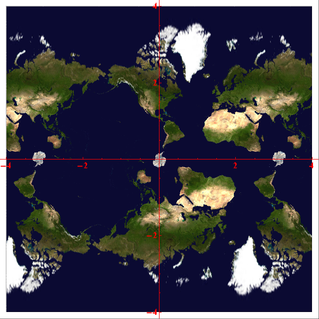
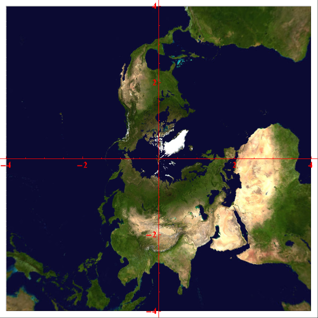
Excited by this prospect, I set to work programming it. The simplest function is the identity function, which gives the following complex plot (apologies for the blurry polar regions; I used a relatively low-resolution image):

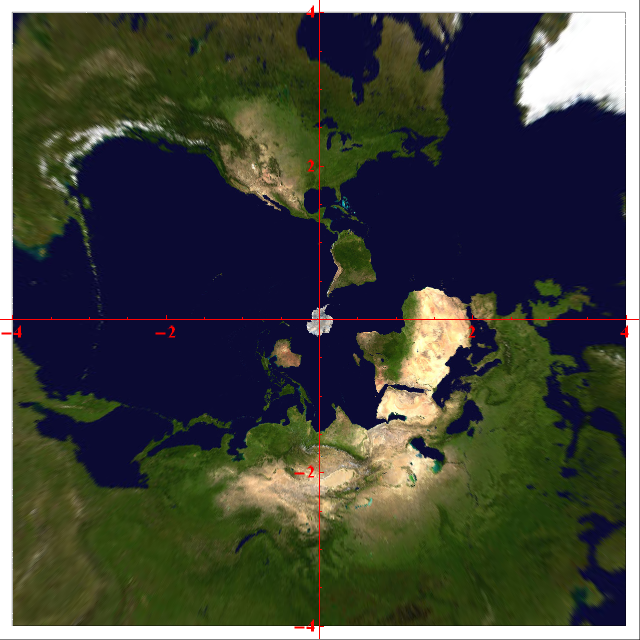
The identity function, f(z) = z

Zeros of functions are rendered as copies of Antarctica. For example, the function f(z) = (z/2)^7 − 1 has seven roots, and thus seven Antarcticas, positioned at the vertices of a regular heptagon of circumradius 2.

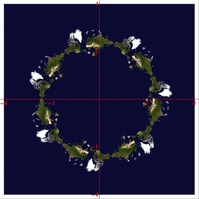
The function f(z) = (z/2)^7 – 1, with seven roots at the vertices of a regular heptagon

It has seven-fold symmetry about the origin since it is a polynomial function of z^7. Similarly, the function f(z) = z^3 has three-fold symmetry, as we can see below:

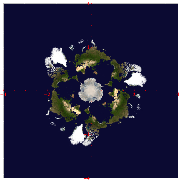
The function f(z) = z^3, with three-fold rotational symmetry and a triple root

Note that the Antarctica in the centre of this plot has three protrusions, rather than just one, due to it being a triple root. This allows one to very easily observe the multiplicity of a root in such a visualisation of the complex plane. For instance, the polynomial f(z) = (z/2 − 1)^2(z/2 + 1)^3 is shown below:

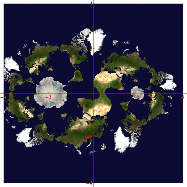
A complex polynomial with a double root at 2 and a triple root at -2

Functions other than polynomials

So far, all of our functions have been polynomials. Other functions, such as sine and cosine, are more interesting due to the infinity of roots:

The function f(z) = sin(z), demonstrating periodicity parallel to the real axis

There are visible copies of Antarctica at −π, 0 and π. The cosine function is the same, but shifted slightly. The two-fold rotational symmetry means that it is an even function:

The function f(z) = cos(z), showing rotational symmetry

We can have more bizarre functions, such as the Gamma function, which have many poles (points mapped to infinity).

The Gamma function, a generalisation of the factorial function, with poles at non-positive integers

The Weierstrass elliptic function has a regular lattice of poles, together with two interleaved lattices of zeros. These appear as Arctic tundras and Antarcticas, respectively.

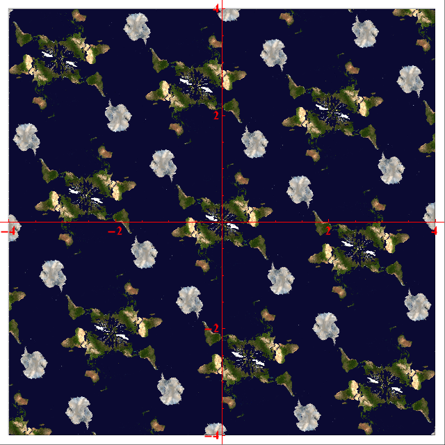
A Weierstrass elliptic function, exhibiting double periodicity

Unfortunately, the poles are rendered poorly due to the texture functionality in Mathematica (it doesn’t realise that the map should be treated as a sphere). I could rectify the situation by using the Image command instead of the RegionPlot, but this would require the use of compiled functions which are not supported on the Wolfram Demonstrations Project.

Non-meromorphic functions

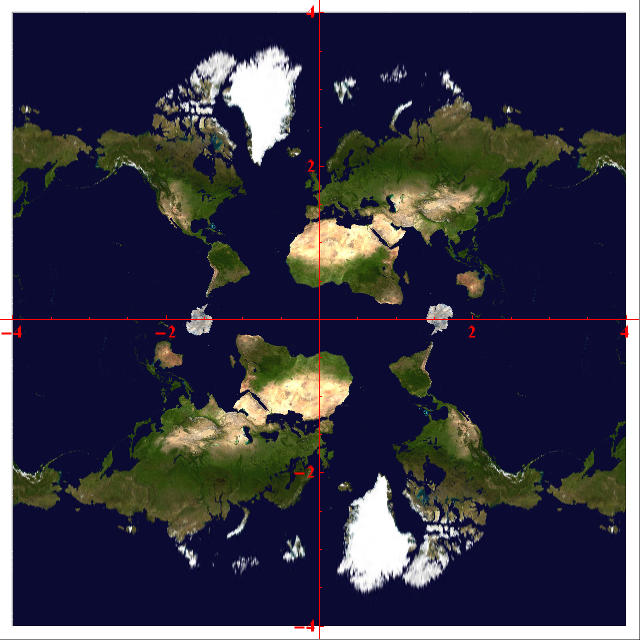
Note that all of the things we’ve seen so far are conformal maps, which preserve angles and orientations. This is a property of all meromorphic complex functions, and means that shapes aren’t locally distorted. If we choose a function which is analytic in the conjugate of z, such as inversion in the circle of radius 2 (f(z) = 4/z*), then the orientations are reversed:

Inversion in the circle |z| = 2

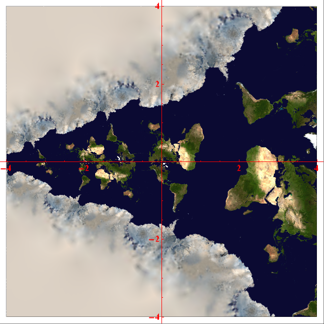
We can tell that this is an anticonformal map, since the British Isles (and everything else!) have been reflected. Worse still are maps which are neither conformal nor anticonformal, since you get weird distortion effects. For example, the absolute value function just has the positive real line as its image, and circles around the origin are mapped to the same value. This creates a ‘target’, where the outermost green band is the intersection of England with the Greenwich Meridian, revolved into an annulus:

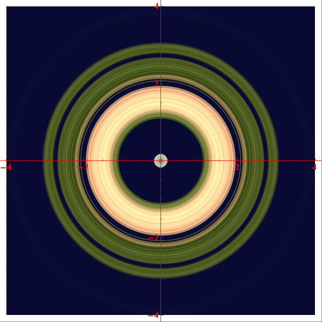
Plot of the absolute value function, f(z) = |z|

Similarly, Re(z) creates vertical lines, and Im(z) creates horizontal lines.