Complex Projective 4-Space

David Smith, Joseph Myers, Craig Kaplan, and Chaim Goodman-Strauss have discovered an aperiodic monotile: a polygon that tiles the plane by rotations and reflections, but cannot tile the plane periodically.

Any tiling induced by the monotile is scalemic: the majority of tiles are unreflected, with only a relatively small proportion (shown in dark blue) being reflected. The ratio of unreflected to reflected tiles is φ^4 : 1, as can be determined from taking the authors’ description of the tiling in terms of a substitution system of ‘metatiles’:

• H → 3H + 3P + 3F + T
• P → 2H + P + 2F
• F → 2H + P + 3F
• T → H

and then taking the dominant eigenvector (corresponding to the dominant eigenvalue φ^4) to find the proportions of metatiles in the limit tiling, and using that to deduce the fraction of unreflected monotiles.

The tile itself is remarkably simple: it is a 13-sided polygon formed from the union of eight of the kites in the deltoidal trihexagonal tiling, which is itself the common refinement of the regular hexagonal tiling and its dual:

Adapted from an illustration by Tilman Piesk

This paper came a few days after the solution of another long-standing open problem in combinatorics, namely an improvement to the exponent in the upper bound on the Ramsey number R(s, s).

Additionally, a few months ago Barnabas Janzer proved that there exists a pair of convex compact sets each homeomorphic to a closed 4-ball such that a copy of S exists inside K in every orientation, but such that (remarkably!) the space of ways to embed copies of S inside K is not path-connected. This resolves a question posed by Hallard Croft.

A couple of years ago I described a prime p which possesses various properties that renders it useful for computing number-theoretic transforms over the field . Specifically, we have:

where the first of these equalities uses the identity that:

where rad(k) is the product of the distinct prime factors of k.

It transpires that at approximately the same time, this field and its properties were rediscovered by the authors of the cryptographic protocol Plonky2. Remco Bloemen has written an article on this prime, which he calls the Goldilocks prime. Remco’s article is very much worth reading; it contains a bunch of new things not present in my original article, such as a fast implementation of modular inversion* based on the binary GCD algorithm, as well as a comprehensive discussion of Schönhage’s trick and some closely related variants.

*which can be improved by a further 20% as implemented here.

Besides convenient real-world properties such as fitting neatly into a machine-sized integer, there are two important mathematical properties of p:

• p − 1 is divisible by , so th roots of unity exist in the field . This supports power-of-two-length NTTs up to length .
• 2 is a primitive 192th root of unity, so multiplying an element of the field by a 192th root of unity (or indeed a 384th root of unity, by Schönhage’s trick) is particularly efficient. Since 192 has a large power-of-2 divisor (64), this means that we can use radix 64 for implementing these NTTs efficiently.

This prime has a much larger cousin with very similar properties:

We’ll call this the Osmiumlocks prime, because it’s in some sense a heavier version of the Goldilocks prime.

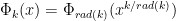
In this case, 2 is a primitive 1600th root of unity, and th roots of unity exist in the field, so we can have extremely large power-of-two-length NTTs. This is very fortuitous, even more so than the Goldilocks prime p, because the reason that k/rad(k) = 160 is so large is because the prime factorisation of k = 1600 = 2^6 . 5^2 has both prime factors repeated.

The beneficial properties of the Osmiumlocks prime q as compared with the Goldilocks prime p are that it’s sufficiently large to use for cryptography (for example, as the base field for an Edwards curve) and that it allows vastly longer power-of-two-length NTTs. You would only be limited by the maximum length of a power-of-two-length NTT over this field if you could store 2^160 words in memory; unless each word could be stored in fewer than 100 atoms, there are insufficiently many atoms inside the planet to build such a machine!

The disadvantage is that, being 640 bits long, field elements no longer fit into a 64-bit machine word. We’ll address this issue shortly.

Also, whereas multiplying by cube roots of unity was efficient in the Goldilocks field, it’s no longer efficient in the Osmiumlocks field; conversely, multiplying by fifth (and, less usefully, twenty-fifth) roots of unity is now efficient whereas it wasn’t in the Goldilocks field. All of the roots of unity in the Goldilocks field still exist in the Osmiumlocks field, though, because q − 1 is divisible by p − 1.

An unlikely alliance

I originally saw these two primes p and q as competitors: two primes with similar properties but very different sizes. It transpires, however, that the properties of p help to address the drawbacks of q, namely its inability to fit into a single machine word.

How would we implement arithmetic modulo q? If we represented it as 640/64 = 10 machine words, then we’d need 100 multiplication instructions (together with carries and suchlike) to implement multiplication using the ordinary method for integer multiplication. Instead, we’ll make use of the following observation:

This means that the field embeds into the ring of integers modulo , so we can do our arithmetic in this larger ring (reducing at the end if necessary). How does that help? If we represent the elements in this ring as degree-n polynomials in a variable , then multiplying the polynomials modulo is just a negacyclic convolution.

If we set n = 32, so that , then the coefficients of the polynomials are 25-bit integers. When we take a negacyclic convolution of two such polynomials, each coefficient will be the sum 32 different 50-bit products, which (allowing for an extra bit to deal with signs) will therefore fit in 56 bits.

We can do this negacyclic convolution efficiently using NTTs if we have efficient 64th roots of unity, which indeed we have in the original Goldilocks field! We can therefore compute one of these length-32 negacyclic convolutions over the Goldilocks field , involving just 32 multiplications of machine integers, a factor of 3 smaller than the 100 we would have otherwise needed.

We’ll need other operations, such as shifts and adds, but these tend to be cheap operations. Whether or not this is worthwhile depends on the size of the hardware multiplier. Many GPUs implement a full 64-bit product as many individual calls to a smaller (16- or 32-bit) hardware multiplier, so there we would experience a greater advantage from this NTT-based approach.

Also, the relevant operations vectorise very well: on a GPU, each warp consists of 32 threads, and we can have the ith thread in a warp hold the coefficient of . Both the NTT butterfly operations and final carrying operations (to reduce the 56-bit coefficients back down to 25 bits) can be efficiently implemented using shuffles, which we have previously used in the context of fast Gaussian random number generation, and any arithmetic operations are performed across all threads in parallel.

In the tensor rank paper we introduced a new family of axis-aligned n-dimensional polytopes, one for each positive integer n. The vertices are naturally identified with ordered partial partitions (OPPs) of {1, …, n}, and the edges correspond to converting one OPP into an ‘adjacent’ OPP by moving an element in a specific way.

Here are the polytopes for n = 2 and n = 3:

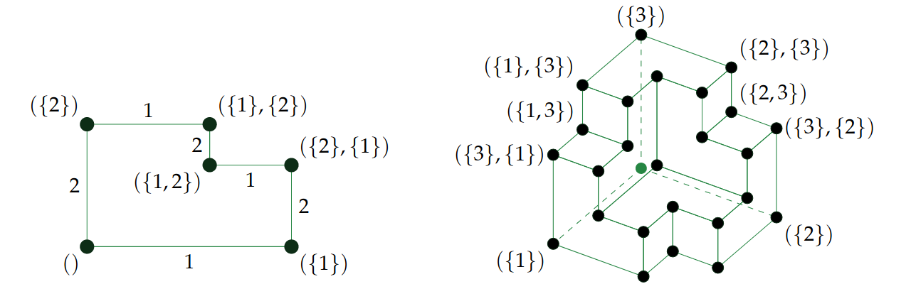
Geometrically, the polytope has a simple description as being the set of all vectors such that, for all k, the kth smallest coordinate is in the interval [0, k]. It has volume and can tile the ambient space by translations.

But this doesn’t shed very much light on the combinatorial structure of the polytope, so it is useful to have a concrete description of the vertices, edges, and higher-dimensional faces. This was introduced in the paper, but the paper was chiefly concerned with the tensor rank of the determinant and therefore we did not delve too deeply into this.

As in the figure above, an ordered partial partition can be described by a list of disjoint subsets. For example, one of the OPPs of {1, …, 8} is:

[{3, 5}, {7}, {1, 4, 8}]

It is ordered because the order of the parts matters, and partial because some elements are allowed to be missing (in this case, 2 and 6). We can also draw this as a diagram where the parts are shown as layers, and all of the absent elements are present in a ‘ground level’ together with a sentinel value 0:

Whilst such a diagram takes up a lot more space, it is more helpful for visualising how an OPP can be transformed into an adjacent OPP. The two allowed moves are:

• Taking a (nonzero) element that is the only occupant of its level (e.g. 7), and ‘merging it down’ into the next level (currently {3, 5}). The total number of levels decreases by 1.
• Taking a (nonzero) element that is not the only occupant of its level (e.g. 2), and ‘separating it up’ into its own new level. The total number of levels increases by 1.

(This description is different from, but equivalent to, the one in the paper: the paper omits the ‘ground level’ and therefore instead has elements disappear and reappear; here we include this ‘ground level’ explicitly to make some of the descriptions more concise.)

For a given element i ∈ {1, …, n}, exactly one of these two moves is possible (depending on whether or not it is the only occupant of its level), and the two moves are inverses of each other.

The polytope and its face lattice

For a fixed n, we define a polytope whose vertices correspond to the OPPs of {1, …, n} and edges join pairs of OPPs if they can be interchanged by moving an element according to the aforementioned rules. Each vertex is incident with n edges, because from each OPP, we can move any of the n elements in exactly one way.

What about the higher-dimensional faces? A k-dimensional face is given by taking an OPP, allowing some size-k subset of the elements to be ‘movable’, and the remaining elements to be ‘immovable’. For example, we might make {2,3,7} movable elements, and the reachable configurations define a 3-dimensional face. Here we show the same OPP as before, but with the movable elements coloured in red:

We have also placed a solid black ‘floor’ on any level that contains an immovable element, because it is impossible for any elements to ever pass through those floors whilst subject to the rules we’ve described.

Which OPPs are reachable from this configuration? The element ‘2’ can stay on the ground level or move up into its own new level, so it has two possible locations. There are six possible configurations for the elements {3, 7}, depending on their relative orderings (3 possibilities) and whether or not at least one of them shares a level with ‘5’ (2 possibilities). Together, that means that this three-dimensional face has 12 vertices (where, by convention, we have omitted the contents of the ground level):

• [{3, 5, 7}, {1, 4, 8}]
• [{3, 5}, {7}, {1, 4, 8}]
• [{5}, {3}, {7}, {1, 4, 8}]
• [{5}, {3, 7}, {1, 4, 8}]
• [{5}, {7}, {3}, {1, 4, 8}]
• [{5, 7}, {3}, {1, 4, 8}]
• [{2}, {5, 7}, {3}, {1, 4, 8}]
• [{2}, {5}, {7}, {3}, {1, 4, 8}]
• [{2}, {5}, {3, 7}, {1, 4, 8}]
• [{2}, {5}, {3}, {7}, {1, 4, 8}]
• [{2}, {3, 5}, {7}, {1, 4, 8}]
• [{2}, {3, 5, 7}, {1, 4, 8}]

We have enumerated them in the order of a Hamiltonian cycle, making it apparent that these are indeed all reachable and therefore form a face of our polytope.

Counting the faces

Note that any face has a unique ‘minimum-energy’ vertex: the ordered partial partition where we merge all movable elements down into the next level containing at least one immovable element. To count the faces in the whole polytope, it therefore suffices to count, for each ordered partial partition, the faces that have that particular OPP as their minimum-energy vertex.

A vertex is minimum-energy if and only if every non-ground level contains at least one immovable element. This means that for a particular ordered partial partition R, the set of movable elements must be chosen by taking some (possibly empty) proper subset of each non-ground level P ∈ R together with an arbitrary subset of the ground level. The generating function of faces with R as its minimum-energy vertex is therefore the polynomial:

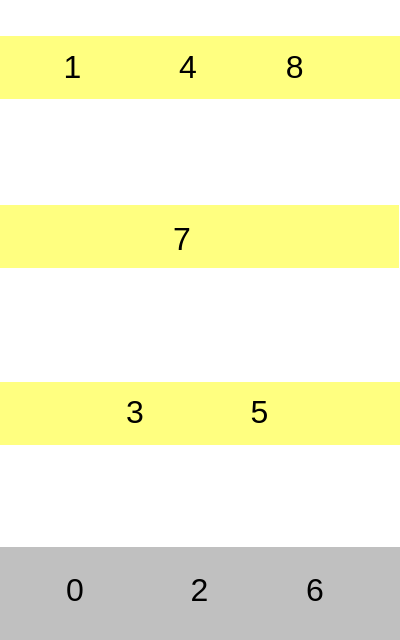
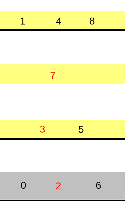
where the coefficient of counts the number of k-dimensional faces with R as its minimum-energy vertex, and m is the number of non-ground elements in R.

To obtain the full face-generating function for the whole polytope, we just need to sum over all ordered partial partitions R. The number of such ordered partial partitions grows superexponentially, which is problematic. However, the polynomial doesn’t depend on the ordering of the parts or the specific choice of elements in each part, so we just need to sum over all partitions of each integer m ≤ n and multiply each polynomial that occurs by the number of ordered partial partitions corresponding to that particular integer partition.

Integer partitions grow subexponentially, so it is much more feasible to count them. Here is some Wolfram Mathematica code that uses this idea to compute the face-generating function for the whole polytope as a function of n:

It’s relatively quick to compute the face-generating function up to n = 30. Here are the values for n up to 8 dimensions:

The constant term counts the number of vertices, given by A000629 in the OEIS. The linear term counts the number of edges; it doesn’t appear to be in the OEIS, but by n-regularity, it’s just n/2 times the number of vertices.

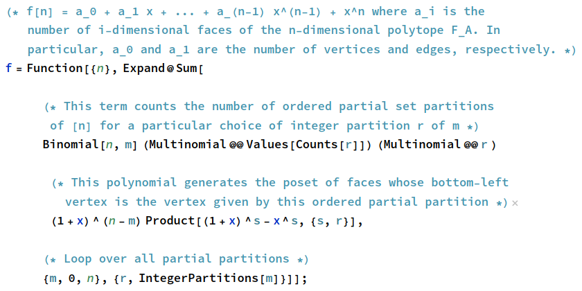
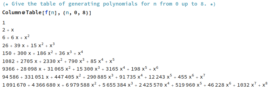
The term in counts the codimension-1 faces, or facets, of the polytope. This sequence is A215149 in the OEIS, and has closed form . We can interpret this geometrically: for each standard basis vector , there are facets with outward normal and one facet with outward normal ; summing over all n of the standard basis vectors gives the result.

The polytopes start to get outrageously complicated for larger n. For example, when n = 30, there are more than 22 undecillion vertices, 342 undecillion edges, and 16 billion facets:

Having a convenient way to compute the k-dimensional faces of the n-dimensional polytope in this family means that this could be submitted to the Encyclopedia of Combinatorial Polytope Sequences, which catalogues objects such as simplices, hypercubes, permutohedra, and associahedra.

An infinite-dimensional polytope

As abstract polytopes, these are nested: every ordered partial partition of {1, …, n} is also an ordered partial partition of {1, …, n+1}. This means that we can take their union, and obtain an abstract infinite-dimensional polytope whose vertices are all finitely-supported ordered partial partitions of the positive integers.

Robin Houston, Nathaniel Johnston, and I have established some new bounds on the tensor rank of the determinant over various fields. The paper is now available as an arXiv preprint and contains the following results:

• A new formula for the determinant (Houston’s identity) which applies over arbitrary commutative rings and establishes an upper bound of the nth Bell number for the tensor rank of the n × n determinant. This is a superexponential improvement over the previous state-of-the-art, which was
• Tighter upper bounds in fields of characteristic p using the same identity, including an upper bound of in characteristic 2.
• Two completely independent proofs of Houston’s identity: a combinatorial proof (which is a more streamlined version of the proof from this cp4space post) and a geometric proof.
• Mildly improved lower bounds on the tensor rank of the determinant (improving Derksen’s bound by a small additive term).
• A computer-assisted proof that the tensor rank of the 4 × 4 determinant over the field of two elements is exactly 12, which consumed 357 core-hours of CPU time*.
• Some geometrical motivation which relates the formula to an interesting tiling of axis-aligned polytopes, the 1-skeleton of which is interpretable as a flip graph for ordered partial partitions:

David Eppstein talks more about orthogonal polyhedra here.

*the same machine later found the Walrus, the first (and currently only known) example of an elementary c/8 diagonal spaceship in Conway’s Game of Life.

At the end of the recent post on a combinatorial proof of Houston’s identity, I ended with the following paragraph:

This may seem paradoxical, but there’s an analogous situation in fast matrix multiplication: the best known upper bound for the tensor rank of 4-by-4 matrix multiplication is 49, by applying two levels of Strassen’s algorithm, but there is a little-known method by Winograd for multiplying two 4-by-4 matrices over a commutative ring using only 48 multiplications.

DeepMind’s AlphaTensor (blog post, Nature article, source code) has since found many non-equivalent 49-multiplication algorithms for 4-by-4 matrix multiplication, as well as improving on the state-of-the-art for some other sizes of matrix multiplication tensor.

As far as I can tell, DeepMind’s new algorithms do not beat the matrix multiplication exponent implied by Smirnov’s incredible algorithm for computing a 3-by-3-by-6 rectangular matrix multiplication using only 40 multiplications:

• Naive exponent: 3
• Strassen exponent: log(7) / log(2) = 2.8074
• Smirnov exponent: log(64000) / log(54) = 2.7743

There are also a few galactic algorithms (which are not used in practice because their advantage over Smirnov only applies to extremely large matrices) which improve the exponent considerably further:

• Coppersmith-Winograd: 2.3755
• Virginia Vassilevska Williams: 2.3729
  

Matrix multiplication in GL(4, 2)

DeepMind’s AlphaTensor also found a record-breaking 47-multiplication algorithm for 4-by-4 matrix multiplication over the finite field . One reason why 4-by-4 matrix multiplication over in particular is interesting is that the group of invertible matrices, GL(4, 2), is isomorphic to the alternating group A_8.

To summarise, here are the various algorithms for 4-by-4 matrix multiplication over (all except the DeepMind algorithm work over arbitrary rings):

• Naive: 64 multiplications + 48 additions;
• Strassen^1: 56 multiplications + 88 additions;
• Strassen^2: 49 multiplications + 165 additions;
• Winograd: 48 multiplications + 120 additions;
• DeepMind: 47 multiplications + ???* additions;

where the DeepMind algorithm can be applied recursively (unlike Winograd) to yield better exponents for large matrix multiplication over this field. Note that multiplications and additions over are individual AND and XOR gates, respectively.  The naive algorithm has the advantage that the circuit has a small number of gates (112) and very low depth (3).

*AlphaTensor finds low-tensor-rank decompositions for tensors, rather than arithmetic circuits, so there’s a subsequent optimisation problem to reduce the number of additions. For example, Strassen’s algorithm for 2-by-2 matrices originally cost 7 multiplications and 18 additions, but the number of additions was later reduced to 15.

In the Treefoil article, I erroneously described John Rickard’s length-24 cycle in as being the ‘uniquely minimal’ example of a cycle whose three axis-parallel projections are all trees (see here for a more detailed history on this problem). Dan Simms has since found a second non-equivalent length-24 cycle with the same bounding box, namely {0, 1, 2}^3. Whereas Rickard’s cycle avoids the central point in that bounding box, Simms’ cycle passes through it.

Simon Tatham has exhaustively searched all such cycles in the larger bounding box {0, 1, 2, 3}^3. Up to symmetry, there are 187075 such cycles of lengths between 24 and 50, enumerated below, confirming that Rickard’s and Simms’ cycles are the only examples of length 24 in this bounding box:

{24: 2,
28: 44,
30: 20,
32: 733,
34: 1481,
36: 5705,
38: 24259,
40: 47875,
42: 57937,
44: 31899,
46: 13920,
48: 2289,
50: 911}

Some of these cycles are visualised on Simon’s webpage.

Optimum Boolean circuit update

In other news, I’ve been busy over the last few months (ergo the sparsity of cp4space articles) revisiting the 5-input 1-output Boolean circuits. In particular, I reused the methodology from the 4-input 2-output search, performing an inductive search (with n ranging up to 11) of all sets of functions obtained as an n-step Boolean chain from five inputs.

What made this possible was the observation that every Boolean function has an invariant — the ‘bias’, or absolute difference between the number of 0s and the number of 1s in the truth table — which is constant across the NPN equivalence class. As such, we can classify sets of functions by the multiset of biases, and use that to divide up our problem space into manageable chunks. This enabled the search to be performed in parallel, and under memory constraints (on a 96-thread 768 GB instance from Amazon Web Services), taking about 5 days of wall-clock time to complete.

This effort both independently checked Donald Knuth’s 2005 result about the number of equivalence classes of functions with each cost, but more helpfully provided all of the minimum-cost circuits for all functions with cost <= 11 (there’s a unique equivalence class of functions with cost 12, represented by the truth table 0x169ae443). It would have been prohibitively expensive to find all cost-12 circuits for 0x169ae443, so I settled on exhaustively searching the tree-shaped circuits for this truth table instead.

The total number of helpful circuits is significantly narrowed down by considering the delay of the circuit: for a fixed gate cost, the next most important utility function is how quickly the output of the circuit is available. Each circuit has a 5-tuple of delays (the length of the longest path from each of the 5 inputs to the output), and we restrict to those circuits which are on the Pareto frontier (i.e. not strictly dominated by another circuit). This enabled the vast majority of circuits to be discarded, leaving just 10.6 million circuits in total for the 616124 equivalence classes of nontrivial functions (the constant function and identity functions are considered trivial since they require 0 gates to implement).

After generating these circuits, they were arranged into a 210 MiB flat file for fast access: the first 8 MiB is a k-perfect hashtable (2^17 buckets of 64 bytes each, where each bucket contains up to 13 different equivalence classes of functions) mapping each function to its cost and an index into the remaining 202 MiB which contains the circuits themselves. I’ve also written a second independent program that reads this flat file and checks the validity of all of the 10.6 million circuits.

Robin Houston recently discovered a rather interesting formula for the determinant of an n-by-n matrix. In particular, the formula improves upon the best known upper bound for the tensor rank of the determinant (viewed as a multilinear map which takes n vectors of dimension n — the rows of the matrix — and outputs the determinant).

Houston also provided a Mathematica notebook which allows you to verify it for a given finite n (fast for n ≤ 6; very slow for larger n). The linked example shows n = 5, for which there are 52 nonzero terms as opposed to the 120 in the standard Laplace expansion of the determinant.

The sum ranges over all partial equivalence relations (PERs) on the set of n elements. The sign of a partial equivalence relation, sgn(~), is the product, over all equivalence classes S, of (−1)^(|S|+1). The size of a partial equivalence relation, |[∼]|, is simply the number of equivalence classes.

The partial equivalence classes containing singleton classes each contribute 0 to the sum, so these terms can be neglected; the remaining terms are in bijective correspondence with the set of all equivalence classes, in other words the nth Bell number. As each term is a product, over all rows, of linear functions of each row, this establishes that the tensor rank of the determinant is upper-bounded by the nth Bell number.

Houston discovered this identity by thinking geometrically in 3 dimensions and then generalising the result; we shall present a combinatorial proof of the same identity. In particular, we show that the expanded formula simplifies to the usual signed sum over all permutations, and do so without involving any geometrical or linear-algebraic properties of the determinant.

Part I: multiplicity of non-permutations

Observe that if you fully expand Houston’s identity, the resulting monomials are of the form where f is some function from {1, 2, …, n} to itself.

Also, from the definition, these functions have the property that if x is a fixed point of f, then there are no other elements y such that f(y) = x. This is a strictly weaker condition than injectivity, so some of these monomials that appear in the expansion do not belong in that of the determinant; we shall therefore need to show that these monomials appear with a coefficient of 0.

Given such a function f, which terms of Houston’s identity contain the corresponding monomial when expanded out? Let’s visualise f as a directed graph on the vertex-set {1, 2, …, n} where each vertex has exactly one outgoing edge and introduce the following terminology:

• Fixed point: a vertex x with f(x) = x (i.e. a self-loop);
• Leaf: a vertex x such that there are no incoming edges, i.e. no y such that f(y) = x;
• Nonleaf: any vertex that is neither a leaf nor a fixed point.

Given such an f, we can characterise precisely the partial equivalence relations ~ which, when viewed as terms in Houston’s identity, give rise to the monomial corresponding to f. In particular, they are those partial equivalence relations ~ which satisfy the following properties:

• If x is a fixed point, then it does not appear in any equivalence class.
• If x and y are nonleaves belonging to the same connected component of the graph, then x ~ y.
• If x is a leaf, then either x ~ f(x) or x does not appear in any equivalence class.

Note that any connected component (other than a self-loop) must contain at least two nonleaves: if x is any vertex in the component, then it follows from the constraints on f that f(x) and f(f(x)) are two distinct nonleaves. Consequently, we can describe a compatible PER with an ordered pair of:

• An equivalence relation R on the set of nontrivial connected components of the graph corresponding to f;
• A (boolean-valued) indicator function ι on the set of leaves of f which specifies which leaves belong to equivalence classes in the PER.

The first term here determines the size of ~ (it’s the same as the size of R). Fixing such an equivalence relation R, the sign of ~ depends on the parity of the number of leaves l such that ι(l) = 1. In other words, if there are any leaves at all, then we have an equal number of positive and negative terms of each size, so they cancel out perfectly.

Part II: multiplicity of permutations

As such, we’ve established that the only monomials that appear with nonzero coefficients are indeed the ones corresponding to permutations! It remains to show that the coefficients are correct, but it means that the analysis is much simpler because we can henceforth assume that f is a permutation. There are no leaves at all, and the nontrivial connected components are cycles.

Letting C be the set of nontrivial cycles, recall that we have a PER ~ corresponding to each equivalence relation R on C. The corresponding term in Houston’s identity has a coefficient of:

where sgn(f) is the sign of the permutation f. Summing over all such R, we get that the overall coefficient of the monomial corresponding to f is:

We want to show that this simplifies to sgn(f). We can rewrite it using Stirling numbers of the second kind:

This sum is the alternating sum of the number of facets of each dimension in a solid permutohedron, so is equal to its Euler characteristic, which is 1 by contractibility. (There’s probably a more direct way to show this using inclusion-exclusion.) As such, it does indeed simplify to sgn(f), thereby establishing the validity of Houston’s identity.

Asymptotics and further discussion

As discussed, Houston’s identity establishes an upper bound of (the nth Bell number) for the tensor rank of the determinant. This asymptotically saves a multiplicative factor of:

over the Laplace expansion, which is a substantial (superexponential!) improvement. The previous state-of-the-art appears to be:

which is merely an exponential improvement over the Laplace expansion.

For practical calculation of large determinants over a field, it is far more efficient (polynomial time instead of superexponential time) to perform Gaussian elimination to reduce the matrix into an upper-triangular form and then simply take the product along the diagonal, so these asymptotics are less interesting in practice.

However, there still may be practical value in using this algorithm for small determinants, especially in applications where a branch-free algorithm is desired and multiplications are expensive. For example, it gives an 8-multiplication formula for a 3-by-3 determinant, instead of the 9 from the Laplace expansion, although the same author later discovered a simpler 8-multiplication formula which uses fewer additions/subtractions.

Can a formula be found using fewer than 8 multiplications? Even though the tensor rank for the 3-by-3 determinant is known to be 5, which implies that any ‘multilinear’ formula costs at least 8 multiplications, there may be a nonlinear formula which accomplishes the task in fewer multiplications.

This may seem paradoxical, but there’s an analogous situation in fast matrix multiplication: the best known upper bound for the tensor rank of 4-by-4 matrix multiplication is 49, by applying two levels of Strassen’s algorithm, but there is a little-known method by Winograd for multiplying two 4-by-4 matrices over a commutative ring using only 48 multiplications.

A pair of people called Pavel have independently developed remarkable automata that last record-breakingly long before halting. In both cases, the number of timesteps that it takes for each automaton to halt is so large that it cannot be written down except using iterated exponentiation. Iterated exponentiation is known as ‘tetration’, so we shall describe these automata as ‘tetrational’.

Busy Beaver record

The first one of these is a 6-state 2-symbol Turing machine by Pavel Kropitz last month which takes approximately:

10^10^10^10^10^10^10^10^10^10^10^10^10^10^10^4.023873729

timesteps to halt (where exponentiation is right-associative, so the rightmost exponentiation is applied first). This is a huge improvement over anything known before May 2022; prior to that, the record was small enough that you could explicitly write down the digits of the number of timesteps (a 36535-digit number).

The lifespan of the new record-holder cannot be stored in floating-point format, but can easily be stored and manipulated in a format called level-index notation. Robert Munafo’s HyperCalc calculator uses this format internally, which is how I was able to get the above approximation from the exact formula:

(3^((3^((3^((3^((3^((3^((3^((3^((3^((3^((3^((3^((3^((3^((3^((3^(4)+7)/8)+21)/8)+7)/8)+23)/8)+7)/8)+21)/8)+7)/8)+23)/8)+7)/8)+23)/8)+7)/8)+21)/8)+7)/8)+23)/8)+13)/8)-11)/2

for the number of ‘1’s left on the tape when the machine halts. This is a lower bound on the number of timesteps that the Turing machine performs, and is tight in the sense that it doesn’t affect the leading digits in the ‘4.023873729…’ at the top of the power-tower.

Shawn Ligocki (who has also held the 6-state 2-symbol Busy Beaver record on a number of occasions, including for two brief 3-day stretches last month!) has written an excellent explanation of how the lifespan of Pavel’s Turing machine was computed.

Compact diehard

In the previous month, Pavel Grankovskiy built a configuration in Conway’s Game of Life which initially fits inside a 104-by-96 bounding box and takes approximately:

10^10^10^10^10^10^10^10^10^1.46179

timesteps to cleanly and completely self-destruct. Here is the configuration, colour-coded by the author to indicate the various parts of the machinery:

The symmetrical object in the southwest corner is a spaceship which travels to the southwest at a speed of c/5 (slightly slower than that of the glider, which travels at c/4). Each side of the spaceship catalyses a ‘sawtooth’ mechanism, where a glider reaching the spaceship is converted into a block which is pulled by subsequent glider pairs.

The lower sawtooth is driven by a continuous gun, causing the blocks to materialise at exponentially sparse intervals (each cycle of materialising a block and pulling it to the origin takes 121 times longer than the previous cycle). The upper sawtooth is driven by the exponentially sparse output of the lower sawtooth, causing the blocks to materialise at tetrationally sparse intervals (each cycle being roughly 121 to the power of the previous cycle). Each time this happens, one of the neon-green objects at the far left of the pattern is deleted, until eventually activating a self-destruction sequence.

The clean self-destruction is accomplished by the salmon and orange objects: the salmon objects were manually placed by the author and ensure that the spaceship is cleanly destroyed from behind; the orange cells were placed by an automated search program which uses beam search to find seeds of destruction for a given input pattern.

Subsequently, various authors have managed to optimise this pattern, adding extra layers to the power tower whilst ensuring that the initial configuration fits within a bounding box with area strictly less than 10000 cells. It seems that the current record-holder has a tower of fourteen 10s followed by a real in the interval [1, 10), so it’s one level below the other Pavel’s Turing machine (not that it’s at all reasonable to compare the lifespan of a 6-state 2-symbol Busy Beaver with that of a sub-10000-cell diehard).

Brett Berger has written an article which discusses the design and history of Pavel’s diehard (there was an earlier design with a single sawtooth mechanism which lasted just over 10^870 timesteps, later optimised by Dean Hickerson up to 10^1595 timesteps).

Brett’s article also discusses a tetrational automaton of his own in a puzzle game called Opus Magnum. That has a lifespan of approximately 10↑↑41 timesteps in Knuth’s up-arrow notation: that is to say, a power-tower of 41 copies of the number 10. This contraption contains two organs called recursive filters, which perform the same duty as the sawtooth mechanisms in Pavel’s diehard.

Beyond tetration

Stacking more recursive filters corresponds to adding more up-arrows. Whilst the recently discovered 6-state 2-symbol Turing machine doesn’t seem to be obviously generalisable in this way, there have been other Turing machines which have taken advantage of this idea for more than a half-decade: in 1964, Milton Green described a family of Turing machines for the busy beaver problem, where the kth machine has 2k + 4 states and takes more than steps to halt (with k up-arrows). In particular, the 10-state machine (k=3) takes more than 3↑↑7625597484987 steps to halt, vastly longer than the other automata that we’ve discussed so far.

The next barrier to break is to progress from these primitive-recursive functions to the Ackermann function (level ω in the fast-growing hierarchy). For the contraptions in Conway’s Game of Life and Opus Magnum, this would involve building an organ which can repeatedly build and stack additional recursive filters.

The researchers with usernames Deedlit and Wythagoras have built Turing machines which achieve levels ω (‘Ackermannian growth’) and ω+1 (‘expandal growth’), including an explicit 15-state machine which consumes the output of the 5-state Busy Beaver record-holder (which leaves 2046 copies of a particular motif on its tape) and uses the other 10 states to boost this to more than timesteps.

Further beyond this is level ε0 in the fast-growing hierarchy, a function that grows so quickly that it cannot be proved total in Peano arithmetic. Wythagoras found an 85-state machine based on the Kirby-Paris hydra that takes more than timesteps to terminate.

Thomas Blok and David Madore have recently made significant progress on the problem of finding rational dodecahedra inscribed in the unit sphere, culminating in an infinite parametric family of solutions.

In particular, Thomas began with the constrained version of the problem that I used to find the first solution: namely where the dodecahedron has an order-8 symmetry group generated by reflections in three orthogonal planes. After stereographic projection, we are left with the following picture:

These solutions are parametrised by six positive rational variables, {a, b, c, d, x, y}, as shown in the image above. Thomas made the observation that if we fix {c, d, x, y} and draw the three green circles, then if they intersect at a common point (a, b), that common point must necessarily be rational.

Consequently, the problem becomes much simpler:

Find positive rationals (x, y, c, d) with y < x < sqrt(c² + d²) such that the circumcircles of the three triangles:

• {(0, −y), (0, y), (x, 0)};
• {(0, y), (−c, d), (c, d)};
• {(x, 0), (c, d), ((c² + d²)/x, 0)};

all mutually intersect at a single point.

David Madore responded to Blok’s MathOverflow question and found a degree-18 polynomial equation in 18 variables expressing the cointersection of three circles defined by 9 points. Madore’s polynomial has 27 873 486 terms, so it is rather unwieldy to manipulate.

With the additional constraint that the 9 points form a 3-by-3 symmetric matrix (thus there are only 12 distinct variables), as is the case for the dodecahedron problem, Madore discovered that the degree-18 polynomial has only 1 980 078 terms and factors as a product of three ‘boring’ degree-4 factors (corresponding to degenerate cases where some points coincide) and an ‘interesting’ degree-6 factor with 720 terms.

Blok substituted the coordinates from the dodecahedron problem into the degree-6 polynomial, obtaining a degree-8 polynomial equation in the variables {x, y, c, d}. Blok observed that it is again reducible, with ‘boring’ factors and a degree-4 ‘interesting’ factor that can be written as:

This is homogeneous, because global scale factors do not affect whether a solution is valid or not. As such, fixing one variable (such as setting y = 1) merely fixes the global scale factor. On the other hand, fixing a second variable (such as setting x = 4) does remove a degree of freedom from the solution space. When fixing x = 4 and y = 1, as suggested, we obtain the following equation in the remaining variables:

Observe that this is a cubic equation rather than a quartic equation. (The same is true if we simultaneously fix c and d instead of x and y.) As such, it has an elliptic curve group law, and we can therefore construct new solutions from existing solutions:

The uppermost point here is the rational solution that was found by computer search. The remaining points in the diagram are generated from that point together with the point at infinity (which, unlike in Weierstrass curves, appears not to be a neutral element). Proceeding in this manner, we can produce infinitely many solutions with fixed x and y provided that we have at least one solution that is not a torsion point on the elliptic curve.

The point at infinity

We observed that the point at infinity does not appear to be a neutral element, so perhaps we can use that to generate solutions without needing an initial solution. In particular, this should work with any choices of x and y.

Note that the equation has two terms:

We can divide both terms by to obtain an equivalent equation:

The first term tends to zero as we approach infinity; the remaining terms are a linear equation in c and d. Consequently, the equation after discarding the first term…

…is precisely the equation of the asymptote λ of the elliptic curve! Intersecting this with the line at infinity gives the point at infinity ∞ on the elliptic curve, at which the line λ is tangent. However, λ must also intersect the curve at another point, P, satisfying P + ∞ + ∞ = 0 (in the elliptic curve group law).

The point P is precisely the point where both terms in the elliptic curve equation vanish:

This is exciting, because it gives us a rational point on the correct component (the unbounded one) of the elliptic curve. Unfortunately, one of the two coordinates is negative, so this is not a valid solution to the dodecahedron problem (if you apply stereographic projection then some of the dodecahedron’s pentagonal faces intersect each other).

However, we can repeat the strategy of drawing a tangent line at this point and letting it reintersect our elliptic curve. This gives the following solution:

which is positive when x ≥ 1.9397y and has a simple expression for the norm:

which, in particular, implies that the points (x, 0) and (0, y) are definitely inside the circle of inversion passing through (c, d). Consequently, not only is this an algebraic solution to the problem, but also it yields a valid geometric solution. The intersection points are given by more complicated rational functions of x and y:

Excitingly, when x and y are the two legs of a Pythagorean triple, the radius of the circle of inversion is itself rational, so we can scale down so that the circle of inversion is the unit circle. That means that, after stereographic projection, the dodecahedron is symmetric under reflection in the three coordinate planes.

Taking the (5, 12, 13) Pythagorean triple, the resulting dodecahedron has the following 20 vertices:

• 4 vertices of the form (0, ±1307215, ±2236392)/2590417;
• 4 vertices of the form (±6274632, 0, ±2787625)/6865993;
• 4 vertices of the form (±64472300514372, ±382579158329275, 0)/387973568586253;
• 8 vertices of the form (±386997531010983823086099699996473688, ±553410551662400041405804573591217100, ±568341850739218062368814809404334875) /882634005124184502065650762315319437;

all of which are rational points on the unit sphere.

Since we can generate Pythagorean triples parametrically, this gives us an infinite parametric family of rational dodecahedra in the unit sphere which are symmetric under reflections in the three coordinate axes.

Is it possible to find rational dodecahedra arbitrarily close to a regular dodecahedron? It seems that this should be the case, because (torsion points notwithstanding) each solution should generate a dense subset of the points on the correct component of the elliptic curve.