I’ve spent the last couple of months tackling the problem of designing an algorithm to rapidly generate high-quality normally-distributed pseudorandom numbers on a GPU. Whilst this may seem quite pedestrian, it turned out to be much more interesting than I’d anticipated: the journey involved Hermite polynomials, generating functions, badly approximable numbers, quasi-Newton methods, and nearest-neighbour spatial queries.
EDIT 2023-01-02: the code and lookup tables are now open-source (MIT-licenced) and included as part of Hatsya’s cpads library.
Traditional methods
There are a few well known methods for producing normally-distributed random numbers from uniformly-distributed inputs.
The simplest approach is to just generate a uniformly-distributed random variable and then apply the inverse CDF of the Gaussian distribution. Unfortunately, the inverse CDF of the Gaussian distribution is not easy to compute; it’s a transcendental function with no closed form, so evaluating it on a computer is difficult: you’d need to use a Taylor series or a Padé approximant with enough terms that the output distribution is sufficiently close (in terms of KL-divergence) to a true Gaussian distribution such that they cannot be easily distinguished.
The other problem with this approach is that the output is a deterministic function of a single uniform input. If the input is a random 32-bit integer, then this generator would only be capable of generating 2^32 different output values.
Even if the input is a random 64-bit integer, it would still have a major problem: any value that it can produce must occur with probability at least 1/2^64. If we generated 2^80 random outputs, then there would be far too many (~ 2^16) outside the interval [−9.5, 9.5] or far too few (exactly zero). On the other hand, a true Gaussian generator should produce an expected 2537 outputs with magnitude greater than 9.5.
A commonly used alternative is the Box-Müller method, which takes a pair of uniform random variables and emits a pair of independent standard Gaussians. It uses the fact that if (x, y) is a bivariate standard Gaussian, then the polar coordinates (r, θ) are independent and have simpler distributions: r² follows an exponential distribution and θ is uniformly distributed in [0, 2π].
Whilst it doesn’t involve anything as exotic as the inverse CDF of a Gaussian distribution, it still requires the computation of a logarithm and a square-root (to determine r) and trigonometric functions (to transform from polar coordinates to Cartesian coordinates), so it is also rather computationally expensive.
There are also algorithms based on rejection sampling, such as Marsaglia’s ziggurat algorithm, which are very performant on scalar architectures (such as CPUs) but less so on vector architectures (such as GPUs) because of the presence of conditional branching.
Algorithms based on summing independent random variables
If you were to neglect the cost of generating the uniform random numbers themselves, then an especially cheap (but low-quality) approximation to a standard Gaussian is obtained by taking 12 random U[0,1] numbers and computing their alternating sum:
A − B + C − D + E − F + G − H + I − J + K − L
This works relatively well, but not fantastically (you can visually distinguish between this probability density function (Irwin-Hall) and the counterpart for a true standard Gaussian):
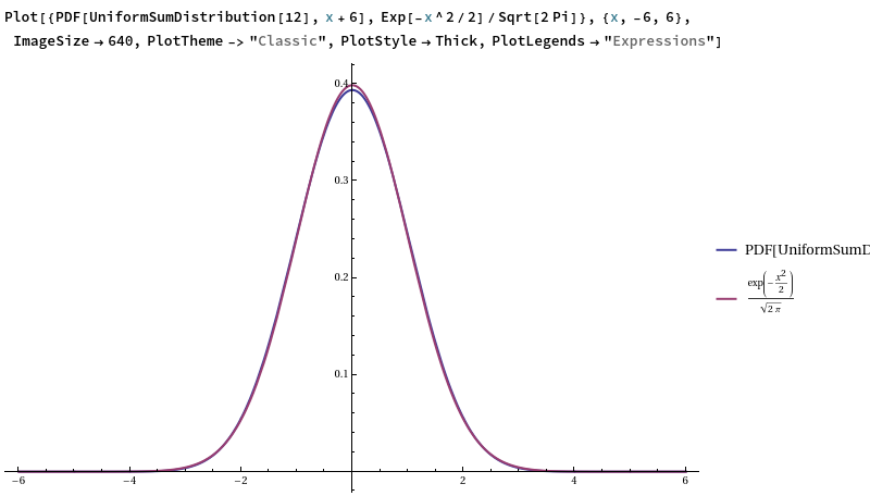
Why is it such a good approximation? Simply put, each uniform random variable has a variance of 1/12, so summing them produces a unit-variance output, and the use of an alternating sum ensures that the output mean is 0. The central limit theorem tells us that summing lots of (finite-variance!) i.i.d. random variables together and rescaling will approximate a Gaussian, and 12 is reasonably close to ‘lots’.
We could improve the quality of the generator by using more uniform inputs, but in reality they’re not free: they have to be produced by a pseudorandom number generator such as PCG or xorwow. Another problem is that it’s far too thin-tailed: the kurtosis of the output is detectably less than 3 (platykurtic), and the number of outputs you need to sample to be sure of that only grows like the square of the number of independent uniforms that you’re summing: so you’d need to sum on the order of 2^20 independent uniforms per output if you want the generator to be able to produce 2^40 outputs before failing the test. Naturally, generating a million uniform random numbers to produce a single output is extremely costly, so the Irwin-Hall method is insufficient for our purposes.
Wallace’s method
Christopher Wallace proposed a stateful method of generating Gaussians, which admits efficient vectorised implementations such as this paper by Brent.
The basic idea is that if you have a set of n i.i.d. Gaussians, then applying an orthogonal matrix in SO(n) produces a different set of n i.i.d. Gaussians (which, of course, are not independent from the first set). Wallace’s generator maintains an internal ‘pool’ of n i.i.d. Gaussians and has the following state-update and output functions:
- State update: apply a sparse random orthogonal matrix to the pool. This is often composed of a permutation and a block-diagonal matrix of Hadamard matrices. Either the permutation or the block-diagonal matrix of Hadamard matrices should be randomised (i.e. depend on bits emitted by a pseudorandom number generator) to ensure that the orthogonal matrix is unpredictable.
- Output function: project down by taking a proper subset of the n Gaussians in the pool. Scale all of these by (the same) random χ²-distributed correction term to correct for the fact that the orthogonal matrix preserves the sum of squared Gaussians in the pool.
To overcome the sparsity of the state-update function and obtain superior mixing properties, one could repeat the state-update function several times between each consecutive output of the generator.
A new algorithm
The key ingredient of Wallace’s generator is the random orthogonal linear transformation that’s applied across the warp to update the state. I then had an idea: what if we use a Wallace-like orthogonal linear transformation not as a state-update function, but as an output function?
As with approaches such as the ziggurat method and Box-Muller, we presuppose that we have a good pseudorandom generator of uniform 32-bit integers, such as Melissa O’Neill’s PCG, and concentrate on the problem of converting this uniformly-distributed input into a normally-distributed output.
In particular, we propose the following architecture:
- each of the 32 threads in the warp generates a uniform pseudorandom 32-bit integer;
- each thread uses some of these input bits to sample two independent weak approximations to a Gaussian, for a total of 64 random variables;
- a random orthogonal linear transformation is applied across the warp to this set of 64 random variables (viewed as a vector in R^64);
- we project down to R^32 by linearly combining the two values in each thread to produce one double-precision floating-point value per thread;
- a small uniform random perturbation is added to the output.
The weak approximations are loaded from a lookup table (using 8 bits of input randomness to load the absolute value from a 256-element lookup table, and a 9th bit to determine the sign). It is necessary to use this lookup table for the weak approximations rather than, say, a uniform distribution, because then our distribution would again be too platykurtic. An alternative could be to use Box-Muller to generate the input distributions, which would be high quality but expensive to compute.
The purpose of the orthogonal linear transformation is twofold: firstly, by the central limit theorem, the marginal distribution of the output is much closer to a Gaussian than the ‘weak approximations’ that we’ve linearly combined; secondly, it aggregates randomness from all 32 of the threads in the warp, so that each output is dependent on 1024 random input bits instead of just 32.
Each of the outputs can each be considered to be a weighted sum of independent random variables, similar to the Irwin-Hall approach where 12 uniform distributions are summed. The orthogonal linear transformation extracts multiple such weighted sums in parallel from the same set of input random variables; the results are non-independent by construction, but the orthogonality of the matrix means that they’re still (linearly) uncorrelated.
Because our approach is stateless (we sample fresh random variables and then apply an orthogonal transformation), we don’t require the annoying χ²-distributed correction term present in Wallace’s generator.
We make a few decisions for efficiency:
- Everything before the final linear projection is done in 32-bit integer arithmetic, with the final linear combination happening in full double-precision floating-point arithmetic.
- The lookup table resides in CUDA shared memory.
- For perfect bank conflict avoidance, thread n only accesses elements of the shared memory array congruent to n (mod 16).
- As such, the shared memory array requires 4096 entries (16 KB), consisting of 16 interleaved lookup tables of 256 entries each.
- There is no reason for these 16 lookup tables to have identical contents, meaning that different residue classes (mod 16) of threads can load different distributions. It transpires that this flexibility does indeed help.
Our random orthogonal linear transformation is a product of sparse matrices, so as to limit the amount of communication between threads. Rather than describe it verbally, it is easiest to draw a dataflow schematic of what happens in each thread. Each of the yellow diamonds is a ‘conditional negate’ operation, which either performs the identity operation or negates its input with probability ½.
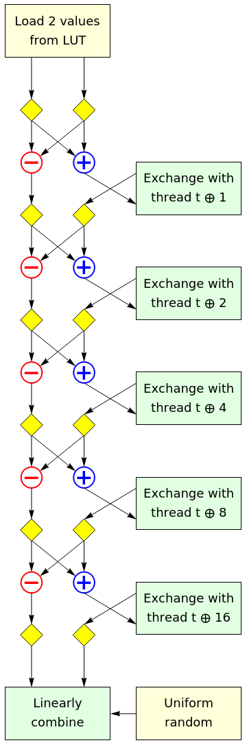
This can be viewed as consisting of 5 copies of the following layer, stacked vertically:
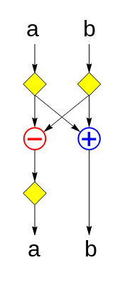
(Technically, if you stacked two of these layers together verbatim, then the ‘a‘ register would have two successive yellow diamonds between the two layers. However, a pair of successive probability-½ negations is functionally equivalent to a single probability-½ negation, so we can ‘fuse’ the two diamonds into one.)
What does this layer do? It uses 3 random bits to uniformly randomly select one of the eight 2×2 Hadamard matrices enumerated below and multiplies it by the input vector (a, b):
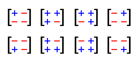
These are, ignoring the scale factor of sqrt(2), precisely the orthogonal transformations where each coordinate of the output depends equally on each coordinate of the input; that is to say, they are ‘maximally mixing’. Omitting the scale factor of sqrt(2) means that this is implementable just using addition/subtraction of integers, and is exact (no rounding errors).
The whole warp performs an FFT-style butterfly network of independent random 2×2 Hadamard matrices; by the end of that process, the ‘a‘ register of a thread contains an equal mix of the 32 input variables from that thread’s half-warp; the ‘b‘ register contains an equal mix of the 32 input variables from the other half-warp. The butterfly network is implemented using the GPU instruction SHFL.BFLY, which is generated by the compiler from the __shfl_xor_sync intrinsic.
Linear combination
Finally, the values in the two registers are linearly combined (in 64-bit floating point, where one register contributes 5/9 of the variance and the other contributes 4/9 of the variance) and an additional low-weight uniform random variable c is added for additional smoothing.
Why are the variance proportions 4/9 and 5/9? They were chosen because the coefficients in the linear combination, 2/3 and sqrt(5)/3, are in the ratio 1 : (φ − ½), which is difficult to approximate with rational numbers whilst still keeping the contributions roughly equal in magnitude.
If the ratio were rational, say in the ratio p : q with small integer coefficients, then the output would be (ap + bq)/f, so the output could only take on discrete integer multiples of f. As such, the output distribution could be distinguished from a Gaussian by looking at the Fourier transform of the distribution — it would have a massive peak at the frequency f and multiples thereof.
The final uniform random variable c is added with a low weight at the very end to further smooth out any high-frequency effects. This is especially important when the output is close to 0, because the absolute precision of an IEEE floating-point number is higher in the neighbourhood of 0; this final perturbation helps to randomise the low-order bits of the mantissa of the output.
How not to populate the lookup tables
My initial idea for populating the 4096-element lookup table was to take the values of the inverse CDF of the Gaussian distribution sampled at 4096 equally spaced points in the interval [½, 1]. This, after all, seemed like a natural way to produce a ‘discrete approximation’ to the Gaussian distribution. This produced the following initial attempt (each row is one of the 16 interleaved distributions).
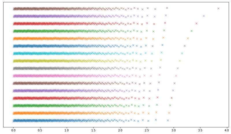
This produced underwhelming results: after generating 2^38 Gaussians using this method and computing the empirical nth moment (mean of X^n) for the first 8 positive integers n, the higher even moments already fail a z-test (we know what the true moments are for a Gaussian, as well as their standard errors).
[----------] 1 test from Gaussian
[ RUN ] Gaussian.Moments
274877906944 trials completed.
moment 1: discrepancy = -2.79812e-06; value = -2.79812e-06
moment 2: discrepancy = -2.41684e-06; value = 0.999998
moment 3: discrepancy = -1.46413e-05; value = -1.46413e-05
moment 4: discrepancy = -0.000106436; value = 2.99989
moment 5: discrepancy = -5.0672e-05; value = -5.0672e-05
moment 6: discrepancy = -0.00155006; value = 14.9984
moment 7: discrepancy = 0.00010665; value = 0.00010665
moment 8: discrepancy = -0.0224637; value = 104.978
[ OK ] Gaussian.Moments (322261 ms)
[----------] 1 test from Gaussian (322261 ms total)
Clearly, we need better ideas.
Optimising the lookup table
The key idea is to note that sampling those 2^38 random Gaussians was actually unnecessary, because we can analytically compute the moments of the distribution produced by our generator. For this initial attempt, we can see that the moment test which fails first is the 8th moment, where the expected time to reach a 4-sigma statistic is 9.1 × 10^10.
However, this realisation that we can analytically compute the expected time to fail the moment tests is our salvation: given a loss function that’s a differentiable function of the 4096 numbers in the lookup table, we can use gradient descent to tweak those numbers to optimise the loss function! We’ll initialise the optimisation with our poor initial attempt and let gradient descent do the rest.
What loss function do we choose? Intuitively, we want the reciprocal of the minimum expected time to fail any of the moment tests. It is, however, important to note that the moments are just expectations E[X^n] of monomials for different powers n, and it may well be the case that there’s a polynomial p such that E[p(X)] provides a more effective test — that is to say, a linear combination of moments is more effective than any individual moment.
Up until now, we’ve been looking at moments, which are the expectations of the elements of the monomial basis {1, X, X^2, X^3, …}. It turns out to be much more elegant to use a different basis, namely the Hermite polynomials:
- He_0(X) = 1
- He_1(X) = X
- He_2(X) = X^2 − 1
- He_3(X) = X^3 − 3X
- He_4(X) = X^4 − 6X^2 + 3
- …
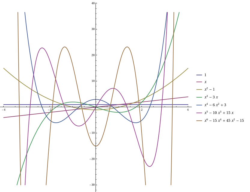
In particular, they are orthogonal polynomials with respect to a standard Gaussian: the expected value E[He_m(X) He_n(X)] is zero when m and n are different, and is n! otherwise. Other than the 0th Hermite polynomial, these all have zero mean, and the covariance matrix Σ is the diagonal matrix whose entries are factorials.
The word ‘moments‘ exists to describe the expected values of powers of a random variable; for brevity, we’ll analogously use ‘hermites‘ (yes, as a plural common noun!) to refer to the expected values of Hermite polynomials of a random variable.
That provides a very convincing choice of loss function: we take log(x^T P x), where P = inv(Σ) is the (conveniently diagonal!) precision matrix of the vector of the first n non-constant even Hermite polynomials under a standard Gaussian assumption, and x is the vector of the first n non-constant even hermites of our approximation of a Gaussian distribution. The inner product x^T P x is proportional to the reciprocal of the worst time to failure of any polynomial test of degree <= 2n.
It turned out to be more numerically viable to optimise the loss function for the simple convolution of the 16 base distributions, even though the actual output of our generator involves more convolutions (the output depends on 64 random variables, 4 from each of the 16 base distributions). These extra convolutions only make the generator better, not worse, so you can view the loss function we’re using as a conservative bound on the generator’s true quality.
We consider a slightly generalised loss function, log(x^T D x) where D is an arbitrary positive-definite diagonal matrix which specifies the relative importance of the different Hermite polynomials.
I used PyTorch as the automatic differentiation framework, so that I only need to implement the forward function and not care about differentiating it myself. PyTorch is chiefly used for training neural networks, where the loss function is too complicated to be symbolically differentiated; instead, it uses ‘reverse-mode’ automatic differentiation (backpropagation).
In order to implement this loss function in PyTorch, it’s necessary to be able to do two things:
- Compute the hermites of a discrete distribution;
- Express the hermites of a linear combination of independent random variables in terms of the hermites of those random variables.
The first of these is easy with the recurrence relation for Hermite polynomials. The second is more involved, and ultimately required discovering what appears to be a new result:
Proposition: Let  with
with  . Then we have:
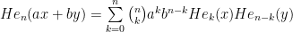
(Observe that when  , this proposition is equivalent to G. Colomer’s first identity mentioned on the MathWorld page. [EDIT: Thanks to Blinkerspawn for pointing out the typo here; I’d originally written sqrt(2) instead of sqrt(2)/2])
Proof: By expanding the binomial coefficient in terms of factorials and pulling out the factor of n!, this is seen to be equivalent to saying that the sequence {He_n(ax + by) / n!} is the convolution of the sequences {a^n He_n(x) / n!} and {b^n He_n(y) / n!}. This is equivalent to saying that the exponential generating function of {He_n(ax + by)} is the product of the exponential generating functions of {a^n He_n(x)} and {b^n He_n(y)}. This generating function is already known, so we can equivalently express this as:

which is indeed true when . QED.
Using this proposition, we can express the hermites of the output distribution (and therefore our loss function) in terms of the hermites of the base distributions, which are in turn obtained from the raw values in the lookup table by means of the recurrence relation.
Then there’s the choice of optimisation algorithm to use. Neural networks often use either stochastic gradient descent or (more recently) Adam, which are great algorithms when we only have an approximate estimate of the loss function (based on a batch of training data). In our situation, though, we can compute the loss function exactly without any noise (floating-point issues notwithstanding).
As such, we instead use the BFGS algorithm as implemented in Reuben Feinman’s torchmin package. BFGS is a quasi-Newton method, maintaining an estimate of the inverse of the Hessian matrix at the current point (based on the history of gradients observed at previously visited points) and using that to determine the next step to take. It mimics true second-order optimisation algorithms such as Newton’s method, but avoids computing the true inverse Hessian at each step (which is very expensive).
Often people use a limited memory variant called L-BFGS, which is helpful if you don’t have enough memory to store a full Hessian matrix. In our case, there are only 4096 parameters, and a 4096×4096 matrix only occupies a very manageable 128 megabytes, so we opted for the original BFGS algorithm instead.
Local search
After this optimisation had converged (requiring occasional small random perturbations along the way to escape saddle points), there was a major problem: the entries in the lookup table are required to be integers, but the optimisation was performed over the reals!
To convert to integers, we multiply by a scale factor of 2^24 and then round to the nearest integer lattice point. This rounding can be quite damaging to the final loss function, so we then perform a local search on the vertices of the 4096-dimensional unit hypercube centred on the unrounded scaled vector, moving to the best vertex within a particular radius of the current vertex until we reach a local optimum.
Our local search algorithm is as follows:
- begin with a starting point (the nearest integer lattice point to the BFGS solution);
- set r = 1;
- for each of the 16 base distributions, try changing r coordinates. If the best improvement (across all 16 × (256 choose r) possibilities) reduces log(x^T D x) by at least 0.001, then move to that new point and jump to step 2;
- if no sufficient improvement was found, increase r (up to a maximum of 5) and jump to step 3;
- if no improvement was found at a local search of depth 5, terminate.
Since x^T D x is a positive-definite quadratic function of x, which is a linear function of each base distribution (when the other 15 distributions are held fixed), we can avoid evaluating (256 choose r) possibilities by instead performing a ball-tree-assisted nearest-neighbour Euclidean search with (256 choose floor(r/2)) query points and (256 choose ceil(r/2)) index points. We use the off-the-shelf implementation in scikit-learn. This gives an approximately quadratic speedup over brute-force, and makes the local search run relatively quickly (for each iteration, the search over all 16 base distributions takes a total of approximately 2 seconds for r = 3, 15 seconds for r = 4, and 90 seconds for r = 5).
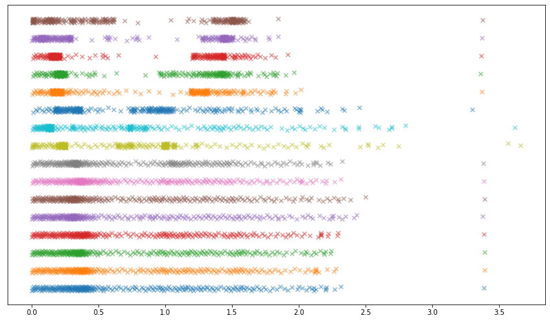
Applying BFGS followed by local search to our initial inverse-CDF-based attempt, we arrive at an unusual set of distributions which yield a considerably better approximation to a Gaussian when convolved:
Choosing the coefficients of a, b, and c
Suppose that we have already populated the lookup tables as detailed in the previous section. Then we can determine the three coefficients by imposing the following constraints:
- the ratio of the coefficients of a and b are sqrt(5) : 2;
- the variance of the output distribution is 1;
- the kurtosis of the output distribution is 3;
where each constraint is understood to mean ‘as close as possible to within floating-point error’.
Since the uniform perturbation is platykurtic (kurtosis less than 3), the random variables a and b need to be slightly leptokurtic (kurtosis greater than 3) in order for this system of constraints to admit a solution. If we can arrange for that to happen, then the output distribution is symmetric (so all odd-order moments are zero) and the 2nd and 4th moments are also correct.
Consequently, when performing the local search mentioned in the previous section, we added a barrier penalty to the loss function to force the convolution of the 16 distributions to be leptokurtic.
The parameters obtained in this manner result in a generator much better than our original attempt: it takes 1.6 × 10^30 outputs in order to fail a moment test at the 4-sigma level, up from 9.1 × 10^10 (the analogous number for the unoptimised distribution).
CUDA implementation
Here is an excerpt of the source code for the generator, minus the contents of the lookup table and the coefficients of a, b, and c in the linear combination. This matches the schematic detailed above, but is more complete as it shows how the random lookups, conditional negation, and final uniform random perturbation are obtained from the 32 bits of input randomness. (The full source code is in the cpads repository.)
#include "stdint.h"
#define _DI_ __attribute__((always_inline)) __device__ inline
#define shuffle_xor(x, y) __shfl_xor_sync(0xffffffffu, (x), (y))
#define COND_NEGATE(i, x) if (entropy & (1u << (i))) { x = -x; }
#define HMIX(i) { int32_t s = a + b; a -= b; b = shuffle_xor(s, i); }

// load the parameters for the random Gaussian generator
#include "parameters.h"

/**
 * Creates a double-precision Gaussian random variable with
 * specified mean and standard deviation. The 'entropy' argument
 * should be a uniform random uint32.
 */
_DI_ double warpGaussian(uint32_t entropy, const int32_t* smem_icdf,
    double mu=0.0, double sigma=1.0) {

    // bank conflict avoidance strategy:
    int laneId = threadIdx.x & 15;

    // use 16 bits of entropy to retrieve two random variables
    // (so the entire warp has 64 such random variables).
    // ....bbbbbbbb........aaaaaaaa....
    int32_t a = smem_icdf[(entropy & 4080) | laneId];
    int32_t b = smem_icdf[((entropy >> 16) & 4080) | laneId];

    // perform the first three layers:
    COND_NEGATE(19, a) COND_NEGATE(18, b)
    HMIX(1)
    COND_NEGATE(17, a) COND_NEGATE(16, b)
    HMIX(2)
    COND_NEGATE(15, a) COND_NEGATE(14, b)
    HMIX(4)
    COND_NEGATE(13, a) COND_NEGATE(12, b)

    // create a uniform random odd int32 (centred on zero).
    int32_t c = (entropy ^ b) | 1;

    // use the lowest 4 bits of entropy (those that contributed the
    // least to the uniform variable c) for the last two layers:
    HMIX(8)
    COND_NEGATE(3, a) COND_NEGATE(2, b)
    HMIX(16)
    COND_NEGATE(0, a) COND_NEGATE(1, b)

    // at this point, a is a {+1,-1}-weighted sum of the 32 values
    // from this half-warp; b is a {+1,-1}-weighted sum of the 32
    // values from the other half-warp.

    double result = mu;

    // our output is the combination of two high-variance Gaussian
    // components and one low-variance uniform component:
    {
        double a_scale = sigma * ordinary_params[0];
        double b_scale = sigma * ordinary_params[1];
        double c_scale = sigma * ordinary_params[2];
        result += a * a_scale;
        result += b * b_scale;
        result += c * c_scale;
    }

    return result;
}
The only ‘surprise’ here should be the way that the uniform random variable c is obtained: it’s the result of XORing the 32 bits of input randomness with the register b and setting the last bit to 1:
int32_t c = (entropy ^ b) | 1;
The value b has just been freshly ‘shuffled in’ from other threads in the warp, so is independent, and because its distribution is symmetric it remains independent even when we conditionally negate it.
Both of these Boolean operations will be fused together in practice, as the CUDA compiler combines them into a ‘LOP3’ instruction — which applies an arbitrary 3-input 1-output bitwise Boolean function specified by a truth table in the form of an 8-bit immediate operand.
Why set the least significant bit to 1? Otherwise, it would be negatively biased (with a mean of −0.5) because the representable 32-bit signed integers are:
{−2^31, −(2^31 − 1), …, −2, −1, 0, 1, 2, … 2^31 − 1}
and the first of these values (bit pattern 0x80000000) ruins the symmetry of the set of representable integers. By setting the least significant bit to 1, we instead have a uniform distribution over the following set of odd integers:
{−(2^31 − 1), …, −5, −3, −1, 1, 3, 5, … 2^31 − 1}
which is symmetrical about 0. We can alternatively view this random variable c as the convolution of 31 Bernoulli random variables with supports:
{−1, 1}, {−2, 2}, {−4, 4}, {−8, 8}, …, {−2^30, 2^30}
which is helpful for analytically computing its moments. (The moments of a small finite distribution are easy to compute, and we can compute the moments of a convolution of two distributions knowing the moments of the original distributions. Because we have to use this idea anyway for the random variables a and b, we may as well use it again for c instead of having to analytically sum a polynomial-valued series.)
We have ignored the subtlety that a and c are not necessarily independent. (b is independent from each of a and c because it originates from the other half-warp.) However, a is conditionally negated according to the least significant bit of entropy, which does not feature in the computation of c (because it was masked out when we bitwise-OR’d the variable with 1), so it follows that a and c have zero linear correlation and also that the output distribution is still symmetrically distributed. Any nonlinear dependence between a and c can only therefore manifest in the 4th moment (and beyond) of the output distribution, where its effect will be negligible because the scale factor applied to c is so small.
Issues with small floats
Let’s assume for the moment that we’re generating standard Gaussians, for which μ = 0 and σ = 1. A slight problem with the generator is that the scale factors of a, b, and c are all multiples of 2^−95, which means that the output is necessarily a multiple of 2^−95.
This only poses an issue for very small outputs: for example, if an output is in the interval [−2^−43, 2^−43], then the lowest bit of the mantissa is forced to be zero. Once we’ve collected (say) 20 outputs in this range, which takes an expected 2.2 × 10^14 samples, then we can be pretty certain that the generator is flawed.
This can be remedied by expressing the scale factor for c as the sum of two double-precision floats instead of as one double-precision float. Then, the last part of our implementation will resemble this:
double result = mu;

{
double a_scale = sigma * ordinary_params[0];
double b_scale = sigma * ordinary_params[1];
double c_scale_hi = sigma * ordinary_params[2];
double c_scale_lo = sigma * ordinary_params[3];
result += a * a_scale;
result += b * b_scale;
result += c * c_scale_hi;
result += c * c_scale_lo;
}

return result;
In doing so, the minimum ‘quantization’ is reduced from 2^−95 to 2^−150, which means that it will take 7.9 × 10^30 outputs to detect the flaw, comparable in magnitude to the moment tests.
It should be stressed that the additional fused multiply-add will slightly slow down the speed of the generator, and it is unlikely to matter for most practical applications of Gaussian random numbers (such as Monte Carlo simulations) where the presence of floating-point rounding errors in downstream calculations are likely of greater effect than the reduced relative precision in the neighbourhood of zero.
Testing with PractRand
Although we have analytically determined that the generator won’t fail any of the moment tests within 10^30 outputs, suggesting that the tail behaviour is correct, there could be other unforeseen problems in the generator. For example, had the coefficients of a, b, and c in the final linear combination been small integer multiples of some common divisor, there would be high-frequency issues with the generated distribution even though the tail behaviour could still be correct.
Consequently, I decided to test this using the PractRand tests following the instructions detailed here. In addition to the suggested patch by Daniel Lemire, it was necessary to change the return type in the declaration of show_checkpoint from ‘double’ to ‘void’, as the function doesn’t actually return anything and was segfaulting when I tried to run it.
PractRand tests that the input is uniformly distributed, whereas the output of the Gaussian generator is supposed to be normally distributed. To test the correctness of the output distribution, it is therefore necessary to apply the CDF of a standard Gaussian distribution to transform it into a supposedly-uniform random variable:
double gaussian = output_host_gauss[i];
double uniform = std::erf(gaussian * 0.7071067811865476);
res[i] = (uint32_t) ((1.0 + uniform) * 2147483648.0);
The error function, erf, produces a uniform random variable in the open interval (−1, 1) when given an input whose probability density function is proportional to exp(x²). Since the probability density function of a standard Gaussian is exp(½x²), it is necessary to divide the standard Gaussian by sqrt(2) before feeding it into the error function. Originally I forgot this factor of sqrt(2), and the PractRand tests reassuringly failed (by a huge margin, with p-values less than 10^−1000) at the first checkpoint.
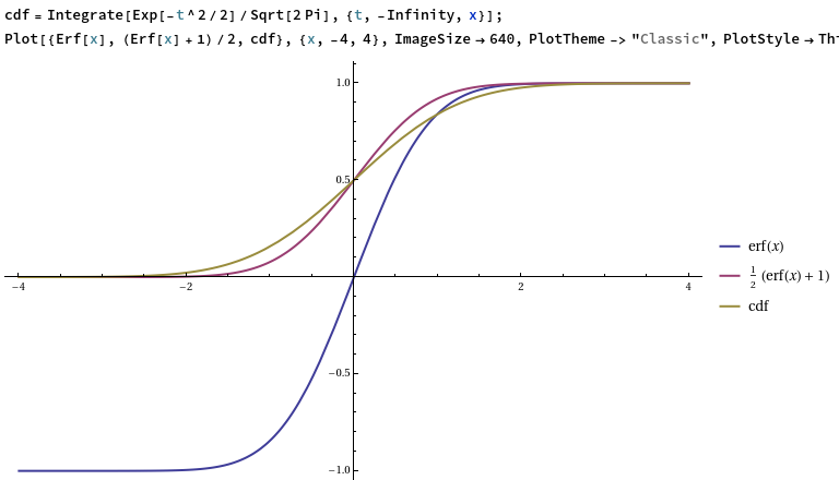
Comparison of the error function, the affine-transformed error function, and the CDF of a standard Gaussian
Then, to convert this into a uniformly random uint32, we apply an affine transformation that maps (−1, 1) to (0, 2^32) and then apply the floor function to the result (implicitly, by casting to an unsigned 32-bit integer).
After running PractRand for approximately four days, the following output was obtained:
$ test/gpu/gpu_gaussian | PractRand/RNG_test stdin32
RNG_test using PractRand version 0.93
RNG = RNG_stdin32, seed = 0xc7ea1bec
test set = normal, folding = standard (32 bit)

rng=RNG_stdin32, seed=0xc7ea1bec
length= 256 megabytes (2^28 bytes), time= 2.7 seconds
no anomalies in 124 test result(s)

rng=RNG_stdin32, seed=0xc7ea1bec
length= 512 megabytes (2^29 bytes), time= 5.6 seconds
no anomalies in 132 test result(s)

rng=RNG_stdin32, seed=0xc7ea1bec
length= 1 gigabyte (2^30 bytes), time= 11.5 seconds
no anomalies in 141 test result(s)

rng=RNG_stdin32, seed=0xc7ea1bec
length= 2 gigabytes (2^31 bytes), time= 22.7 seconds
Test Name Raw Processed Evaluation
[Low1/32]FPF-14+6/16:(4,14-2) R= +6.3 p = 2.7e-5 unusual
...and 147 test result(s) without anomalies

rng=RNG_stdin32, seed=0xc7ea1bec
length= 4 gigabytes (2^32 bytes), time= 45.0 seconds
no anomalies in 156 test result(s)

rng=RNG_stdin32, seed=0xc7ea1bec
length= 8 gigabytes (2^33 bytes), time= 89.9 seconds
Test Name Raw Processed Evaluation
Gap-16:B R= +4.0 p = 2.5e-3 unusual
...and 164 test result(s) without anomalies

rng=RNG_stdin32, seed=0xc7ea1bec
length= 16 gigabytes (2^34 bytes), time= 178 seconds
no anomalies in 172 test result(s)

rng=RNG_stdin32, seed=0xc7ea1bec
length= 32 gigabytes (2^35 bytes), time= 353 seconds
no anomalies in 180 test result(s)

rng=RNG_stdin32, seed=0xc7ea1bec
length= 64 gigabytes (2^36 bytes), time= 707 seconds
no anomalies in 189 test result(s)

rng=RNG_stdin32, seed=0xc7ea1bec
length= 128 gigabytes (2^37 bytes), time= 1406 seconds
Test Name Raw Processed Evaluation
[Low1/32]DC6-9x1Bytes-1 R= -4.2 p =1-6.2e-3 unusual
...and 195 test result(s) without anomalies

rng=RNG_stdin32, seed=0xc7ea1bec
length= 256 gigabytes (2^38 bytes), time= 2785 seconds
no anomalies in 204 test result(s)

rng=RNG_stdin32, seed=0xc7ea1bec
length= 512 gigabytes (2^39 bytes), time= 5625 seconds
no anomalies in 213 test result(s)

rng=RNG_stdin32, seed=0xc7ea1bec
length= 1 terabyte (2^40 bytes), time= 11165 seconds
no anomalies in 220 test result(s)

rng=RNG_stdin32, seed=0xc7ea1bec
length= 2 terabytes (2^41 bytes), time= 22407 seconds
no anomalies in 228 test result(s)

rng=RNG_stdin32, seed=0xc7ea1bec
length= 4 terabytes (2^42 bytes), time= 45386 seconds
no anomalies in 237 test result(s)

rng=RNG_stdin32, seed=0xc7ea1bec
length= 8 terabytes (2^43 bytes), time= 90285 seconds
no anomalies in 244 test result(s)

rng=RNG_stdin32, seed=0xc7ea1bec
length= 16 terabytes (2^44 bytes), time= 213575 seconds
no anomalies in 252 test result(s)

rng=RNG_stdin32, seed=0xc7ea1bec
length= 32 terabytes (2^45 bytes), time= 395812 seconds
no anomalies in 260 test result(s)
There are no test failures here, nor anything suspicious. Occasionally certain tests are encountered with p-values around 0.0001 or 0.9999 and marked ‘unusual’, but they are not too surprising since thousands of tests are performed in total: these ‘unusual’ results are merely green jelly beans.
Tail tests and measuring the speed of the generator
The GPU can generate random Gaussians much more quickly than they can be copied over the PCI-express cable and analysed by PractRand on the CPU. Consequently, we consider a modified tail test, where we copy only the Gaussians whose absolute value exceeds 4. We expect the convolutions to smooth out the behaviour of the distribution in the bulk, so the tails are worth testing more thoroughly.
Only one out of 15787 Gaussians are expected to fall in these tails, so we can better match the relative throughput of the Gaussian generation on the GPU and PractRand analysis on the CPU.
We account for this when mapping to a uniform distribution:
std::vector<uint32_t> retrieve() {
    pcie();
    run_kernel();

    std::vector<uint32_t> res(output_host_count[0]);

    for (size_t i = 0; i < res.size(); i++) {
        double gaussian = output_host_gauss[i];
        double uniform = std::erf(gaussian * 0.7071067811865476);

        if (uniform > 0) {
            uniform -= 0.9999366575163338;
        } else {
            uniform += 0.9999366575163338;
        }

        // map to interval (0, 2)
        uniform = uniform * 15787.192767323968 + 1.0;

        res[i] = (uint32_t) (uniform * 2147483648.0);
    }

    return res;
}
Running this on a Volta V100 produces the following output:
$ test/gpu/gpu_gaussian_tail | PractRand/RNG_test stdin32
RNG_test using PractRand version 0.93
RNG = RNG_stdin32, seed = 0x6f2e57d4
test set = normal, folding = standard (32 bit)

rng=RNG_stdin32, seed=0x6f2e57d4
length= 128 megabytes (2^27 bytes), time= 4.2 seconds
no anomalies in 117 test result(s)

rng=RNG_stdin32, seed=0x6f2e57d4
length= 256 megabytes (2^28 bytes), time= 9.1 seconds
no anomalies in 124 test result(s)

rng=RNG_stdin32, seed=0x6f2e57d4
length= 512 megabytes (2^29 bytes), time= 17.8 seconds
Test Name Raw Processed Evaluation
BCFN(2+0,13-1,T) R= -6.5 p =1-2.9e-3 unusual
...and 131 test result(s) without anomalies

rng=RNG_stdin32, seed=0x6f2e57d4
length= 1 gigabyte (2^30 bytes), time= 35.7 seconds
no anomalies in 141 test result(s)

rng=RNG_stdin32, seed=0x6f2e57d4
length= 2 gigabytes (2^31 bytes), time= 70.9 seconds
no anomalies in 148 test result(s)

rng=RNG_stdin32, seed=0x6f2e57d4
length= 4 gigabytes (2^32 bytes), time= 140 seconds
no anomalies in 156 test result(s)
In particular, it takes 140 seconds to produce 4 gigabytes of output, or equivalently 2^30 outputs (they’re converted to uint32s before piping into PractRand). However, these 2^30 outputs were subsampled from approximately 15787 times as many Gaussians (because we did the 4-sigma tail threshold), so the GPU is actually generating 121 billion Gaussians per second.
121 billion double-precision floats together occupy 968 GB, so it’s producing Gaussian random numbers faster than the Volta can even load/store to global memory (900 GB/s). In other words, it’s faster to run this (in whatever Monte Carlo simulation kernel is consuming the random Gaussians) than it is to load precomputed random Gaussians from the GPU’s global memory.
The GPU is running at full utilisation and PractRand is only showing a long-term average of 37% CPU usage, so (thanks to the tail thresholding) we’re no longer limited by the speed of PractRand. Let’s check up on the PractRand results:
rng=RNG_stdin32, seed=0x6f2e57d4
length= 8 gigabytes (2^33 bytes), time= 281 seconds
no anomalies in 165 test result(s)

rng=RNG_stdin32, seed=0x6f2e57d4
length= 16 gigabytes (2^34 bytes), time= 562 seconds
no anomalies in 172 test result(s)

rng=RNG_stdin32, seed=0x6f2e57d4
length= 32 gigabytes (2^35 bytes), time= 1116 seconds
no anomalies in 180 test result(s)
So far this has consumed about 20 minutes on an AWS p3.2xlarge instance, so roughly $1 of compute to generate a total of 136 trillion Gaussians (7 femtodollars per Gaussian!) and test the approximately 8 billion of those that land in the 4-sigma tails.
Consequently, to run PractRand to its default limit of 2^45 bytes on this tail test would take a fortnight and cost roughly $1000, so I’m loath to run it all the way to completion. Let’s instead stop at two terabytes, which takes nearly 20 hours ($60 on AWS):
rng=RNG_stdin32, seed=0x6f2e57d4
length= 64 gigabytes (2^36 bytes), time= 2238 seconds
no anomalies in 189 test result(s)

rng=RNG_stdin32, seed=0x6f2e57d4
length= 128 gigabytes (2^37 bytes), time= 4468 seconds
no anomalies in 196 test result(s)

rng=RNG_stdin32, seed=0x6f2e57d4
length= 256 gigabytes (2^38 bytes), time= 8899 seconds
no anomalies in 204 test result(s)

rng=RNG_stdin32, seed=0x6f2e57d4
length= 512 gigabytes (2^39 bytes), time= 17848 seconds
no anomalies in 213 test result(s)

rng=RNG_stdin32, seed=0x6f2e57d4
length= 1 terabyte (2^40 bytes), time= 35668 seconds
Test Name Raw Processed Evaluation
[Low1/32]Gap-16:A R= -3.9 p =1-2.5e-3 unusual
...and 219 test result(s) without anomalies

rng=RNG_stdin32, seed=0x6f2e57d4
length= 2 terabytes (2^41 bytes), time= 71144 seconds
no anomalies in 228 test result(s)
Conclusions and acknowledgements
Between these empirical tests and theoretical analysis, it appears that this is a suitable method of generating non-cryptographic pseudorandom normally distributed random variables on a GPU, particularly suited for computationally intensive scientific and industrial applications such as Monte Carlo simulations.
It should not be used for cryptographic applications: there has been no attempted cryptanalysis of the output function, and based on the simplicity of the construction it is likely to be vulnerable to cryptanalytic attacks. Without the linear projection at the end, it would be especially trivial to invert; given the final a and b registers of all threads in a warp, it’s possible to determine (with about 2^32 effort) the random Hadamard transformation, the values loaded from the lookup table, and therefore the lower 28 bits of the input entropy.
If you need cryptographic random Gaussians (for RLWE, for instance) then you should use Dwarakanath and Galbraith’s paper instead.
Finally, many thanks go to Rajan Troll for relevant discussions over the last two months that immensely helped with developing this random Gaussian generator.


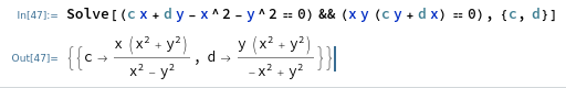
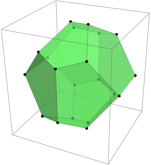
 as being the ‘uniquely minimal’ example of a cycle whose three axis-parallel projections are all trees (see
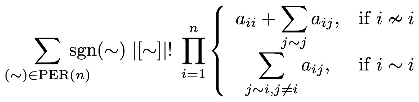
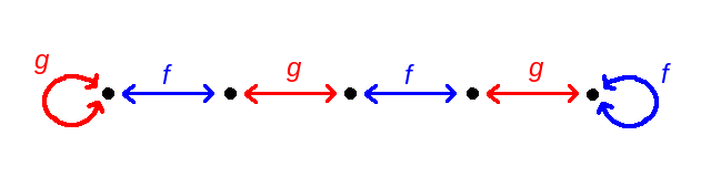
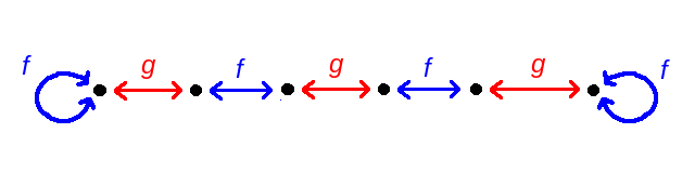
 where f is some function from {1, 2, …, n} to itself.
![|[\sim]|! \textrm{ sgn}(\sim) = |[R]|! \textrm{ sgn}(R) \textrm{ sgn}(f)](https://s0.wp.com/latex.php?latex=%7C%5B%5Csim%5D%7C%21+%5Ctextrm%7B+sgn%7D%28%5Csim%29+%3D+%7C%5BR%5D%7C%21+%5Ctextrm%7B+sgn%7D%28R%29+%5Ctextrm%7B+sgn%7D%28f%29&bg=ffffff&fg=000&s=0&c=20201002)
![\textrm{ sgn}(f) \sum_R |[R]|! \textrm{ sgn}(R)](https://s0.wp.com/latex.php?latex=%5Ctextrm%7B+sgn%7D%28f%29+%5Csum_R+%7C%5BR%5D%7C%21+%5Ctextrm%7B+sgn%7D%28R%29&bg=ffffff&fg=000&s=0&c=20201002)

 (the nth Bell number) for the tensor rank of the determinant. This asymptotically saves a multiplicative factor of:
![(\sqrt[3]{1.2})^n](https://s0.wp.com/latex.php?latex=%28%5Csqrt%5B3%5D%7B1.2%7D%29%5En&bg=ffffff&fg=000&s=0&c=20201002)
 steps to halt (with k up-arrows). In particular, the 10-state machine (k=3) takes more than 3↑↑7625597484987 steps to halt, vastly longer than the other automata that we’ve discussed so far.
 timesteps.
 timesteps to terminate.
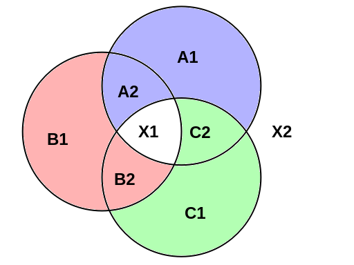
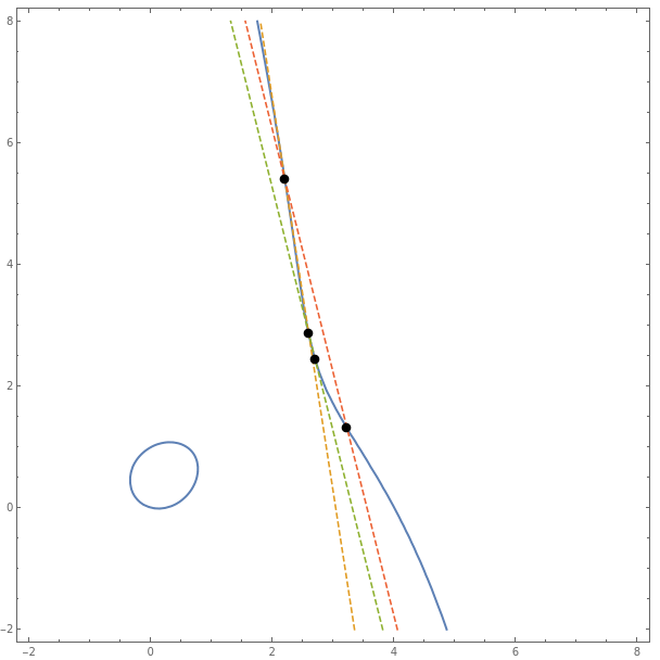
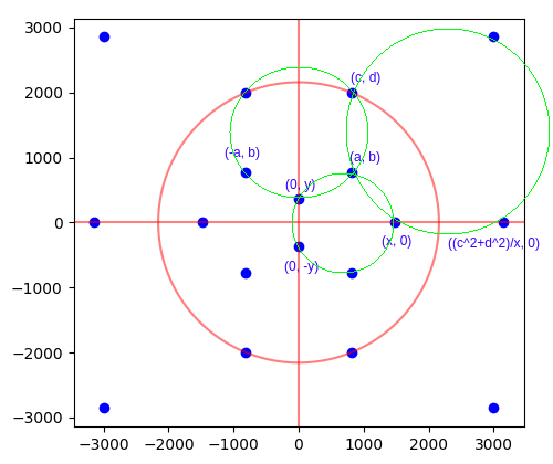 These solutions are parametrised by six positive rational variables, {a, b, c, d, x, y}, as shown in the image above. Thomas made the observation that if we fix {c, d, x, y} and draw the three green circles, then if they intersect at a common point (a, b), that common point must necessarily be rational.
 and a degree-4 ‘interesting’ factor that can be written as:

 to obtain an equivalent equation:


 and the inner field is isomorphic to
  and inner field
  where
where  is a Mersenne prime.
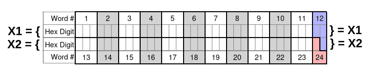
 .
.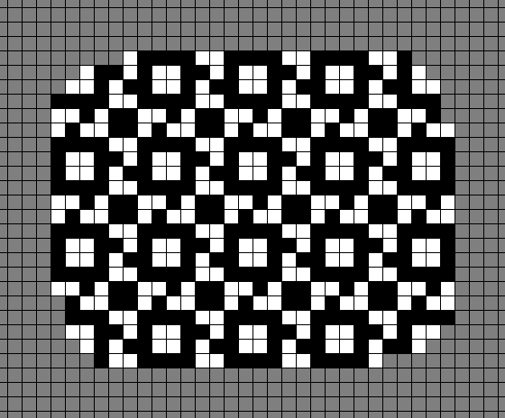
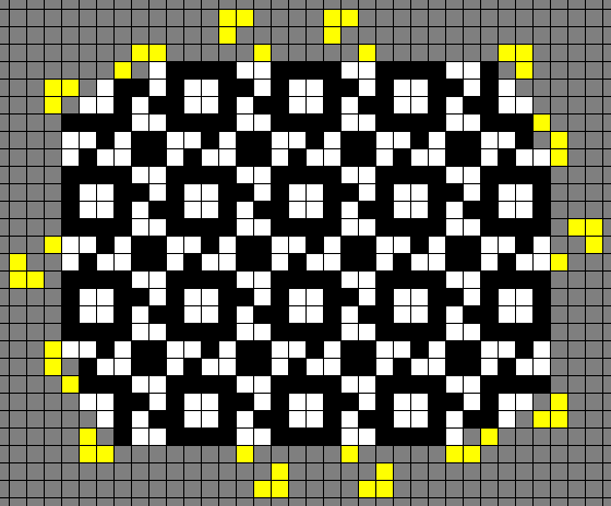
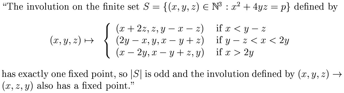
 , and the set U is the singleton set containing the fixed point of the complicated involution g.