
In 1995, William Jockush, Peter Shor and James Propp published the statement and proof of the celebrated Arctic Circle Theorem. This roughly states that if you choose a random domino tiling of an Aztec diamond (a particular family of polyominoes), the resulting pattern is homogeneous outside a central chaotic disc-shaped region:
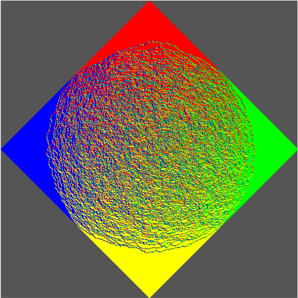
In the diagram above, the colours indicate the orientation and parity of the dominoes. We can now state the theorem more precisely:
- Let ε > 0 and p < 1. Then we can find n such that with probability at least p, the boundary of the disordered region in the centre of a randomly-chosen domino tiling of the order-n Aztec diamond will be contained in the annulus bounded between the concentric discs of radii (1 ± ε)r, where r is the radius of the circle inscribed in the diamond.
Firstly, it is by no means obvious how many domino tilings exist (although one could theoretically bash it with the permanent-determinant method), nor how to efficiently choose a tiling randomly such that all tilings occur with equal probability. The authors of the paper settle both of these issues simultaneously with the shuffling method illustrated below:
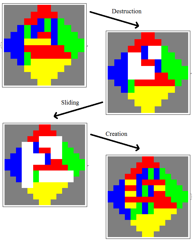
Each domino is given a heading (one of the four cardinal directions) according to the following rules:
- Place a dot in the centre of the uppermost edge of the Aztec diamond.
- Place dots on any other lattice points of the same parity as the original dot.
Then each domino has a dot in the centre of precisely one of its four edges; this determines the heading of the domino. We have used red, green, yellow and blue to represent north, east, south and west, respectively. Each iteration of the shuffling method comprises three stages:
- Destruction: If a pair of dominoes face each other, they annihilate.
- Sliding: All dominoes move one step according to their headings.
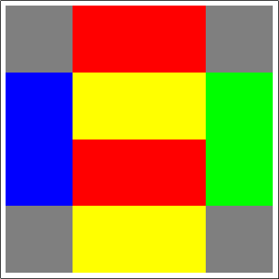
- Creation: Empty cells form the disjoint union of 2-by-2 blocks. Insert two dominoes into each of these blocks in one of two ways (chosen randomly by the result of an unbiased coin toss).
This converts an order-n Aztec diamond tiling into an order-(n + 1) Aztec diamond tiling. Iterating from the base case of a 2-by-2 block, we can obtain any Aztec diamond tiling in this manner. The following animation shows the expansion of a tiling by iterated application of the shuffling method:
This is quite remarkable, as it is surprising that the result of a stochastic process on a square lattice would give rise to a perfect circle. In particular, cellular automata very rarely exhibit this feature (certain lattice gases possess this desired isotropy, but most do not), and tend to have either square or octagonal envelopes of propagation.
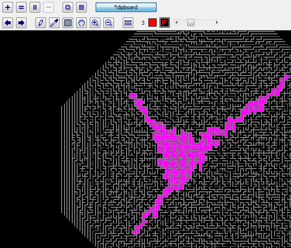
In the comments of the post about the permanent-determinant method, Sam Cappleman-Lynes and I discussed a bijection between domino tilings and spanning trees of the grid graph. Applying the bijection to the result of the shuffling method yields randomly-generated circular mazes which are (given appropriate boundary conditions) simply-connected:
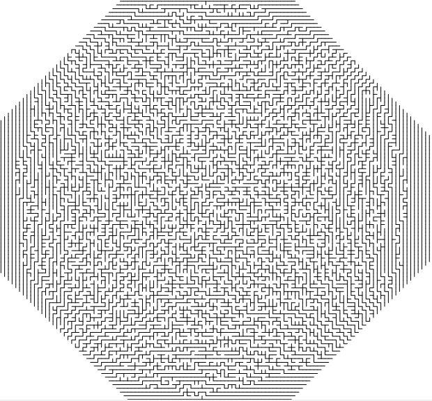
I’m interested in seeing the shortest path from the centre to the boundary, to roughly assess the difficulty of the maze. Now, the obvious thing to try is to run it in the old MazeSolver rule I wrote for Golly, which finds that the maze is rather poorly connected. In particular, routes tend to be pretty direct and very diagonal:
However, this problem only arises due to the fact that we haven’t applied any boundary conditions to the circumference of the chaotic disc. Doing this properly yields a more respectable labyrinth.
your blog is very nice. by the way, do you have a copy the C/C++ code for the aztec domino shuffling algorithm? could you share it?