
Important note: whenever log is mentioned in this particular post, it is referring to the ceiling of the base-2 (binary) logarithm. (Elsewhere on cp4space, when there isn’t this disclaimer, it refers to the base-e (natural) logarithm.)
For reasons that shall soon become clear, I found myself faced with the task of sorting a list of 12 objects.
Usually one would choose an algorithm such as quicksort or Timsort. Conventional comparison-based sorting algorithms operate by comparing pairs of objects, and are otherwise unrestricted: the choices of objects to compare can depend on the results of previous comparisons.
A sorting network is a much more restricted sorting algorithm, where the only allowed operation is the compare-exchange instruction CMPX(i, j). This compares objects in positions i and j, swapping them if they are in the wrong order, and revealing no information. Here are the best known sorting networks on 9 and 12 elements, photographed from The Art of Computer Programming by Donald Knuth:
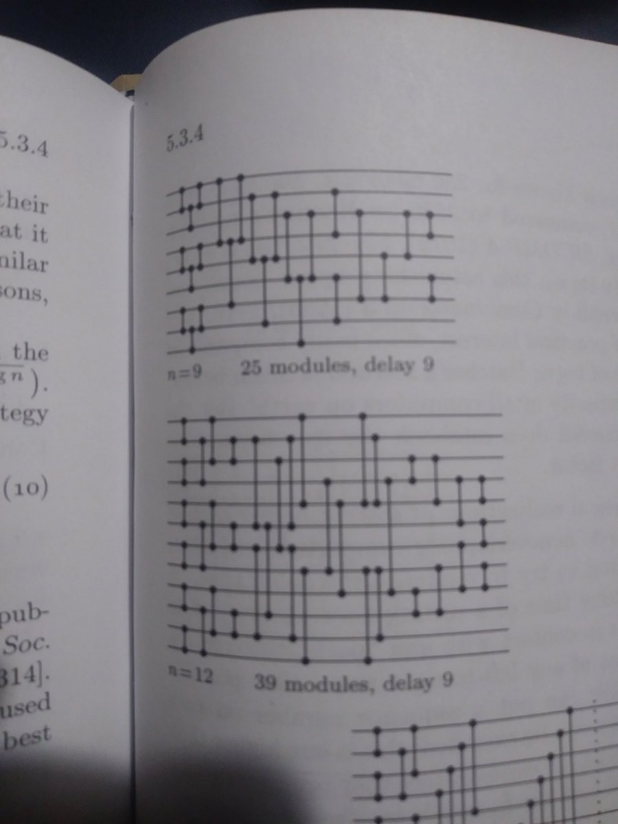
So, with straight-line code of 39 CMPX instructions it is possible to sort a collection of 12 objects without any need for loops, conditional branching, or any other form of control flow. This is especially useful when programming a GPU, where control flow is toxic for performance.
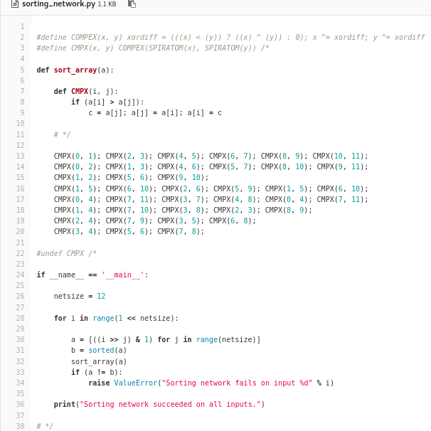
I proceeded to transcribe the sorting network from the above diagram into CUDA code. As a mere mortal, I was not totally convinced that I’d copied it flawlessly, so resorted to building a test to verify the correctness of the transcribed network. Preferring to do this in a high-level language such as Python, I resorted to my usual tricks of writing a single file which is valid in two languages and incorporating it into the source code by means of one innocuous line: #include “sorting_network.py”
(If you think this is bad, people have done much worse…)
Examining the Python component of the code, you may notice that it only tests the 2^12 different binary sequences, rather than the 12! different totally ordered sets. It is a general property of comparator networks that it suffices to only test binary sequences to prove that the network can sort arbitrary sequences; this is known as the 0-1 principle.
Batcher’s bitonic mergesort
What is the minimum number of CMPX gates necessary to sort n objects? And what is the minimum circuit depth? The naive algorithm of bubble sort shows that a gate-count of O(n^2) and a circuit depth of O(n) are both attainable. Similarly, the gate-count must be at least the binary logarithm of n! (as with any comparison-based sorting algorithm) which gives a lower bound of Ω(n log n) for the gate-count and Ω(log n) for the depth.
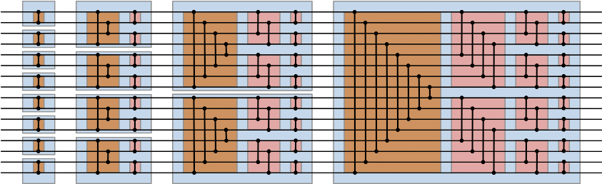
Batcher found a recursive construction of sorting networks with a depth of ½k(k+1), where k is the ceiling of the binary logarithm of n, and each layer has ½n comparators. This is achieved by firstly Batcher-sorting the initial and final halves of the sequence, followed by interleaving them (diagram by User:Bitonic from Wikipedia):
The correctness of the algorithm follows from the aforementioned 0-1 principle. By the inductive hypothesis, it suffices to examine the rightmost blue box and suppose that the two halves of the input are correctly sorted, in which case the input would resemble:
[n/2 – m zeroes] [m ones] | [l zeroes] [n/2 – l ones]
The only ‘cross-lane’ operations are the comparators in the brown box. If l is no greater than m, the result of this is the following:
[n/2 – m zeroes] [m – l ones] [l zeroes] | [n/2 ones]
and otherwise we get the complementary arrangement:
[n/2 zeroes] | [m ones] [l – m zeroes] [n/2 – l ones]
Concentrating only on the non-constant half, our task is reduced to the simpler problem of sorting a binary sequence which switches at most twice between a run of zeroes and a run of ones. We can split the effect of the pink box into two modules: one which reverses one of the two halves (we get to decide which half!), followed by one which behaves identically to a brown box. Observe that, as before, one of the two halves of the pink box must therefore be constant, and the other must again be a binary sequence which switches at most twice. By induction, the result follows.
Owing to the low depth, simplicity, and efficiency, Batcher’s bitonic mergesort is often used for sorting large lists on GPUs.
Beyond Batcher
But is the bitonic mergesort optimal? The circuit above takes 80 comparators to sort 16 inputs, whereas the best circuit in Knuth takes only 60 comparators (again with a depth of 10). It’s not even optimal for depth, as the next page of Knuth has a 61-comparator sorting network with a depth of 9.
What about asymptotics? The bitonic mergesort gives an upper bound on the depth of O((log n)^2) and basic information theory gives a lower bound of Ω(log n).
The next surprise was when Szemeredi, Komlos and Ajtai proved that the lower bound is tight: they exhibited a construction of sorting networks of optimal depth O(log n). As you can imagine from Szemeredi’s background in combinatorics and extremal graph theory, the construction relies on a family of graphs called expanders.
A simplified version of the construction (by Paterson, 1990) is described here. The original paper provides explicit constants, showing that a depth ~ 6100 log(n) is possible, compared with ~ ½ log(n)^2 for Batcher’s bitonic mergesort. In other words, the threshold for switching from bitonic mergesort to Paterson’s variant of AKS occurs when n is approximately 2^12200.
A further improvement by Chvatal reduces the asymptotic constant from 6100 to 1830, and actually provides an explicit (non-asymptotic) bound: provided n ≥ 2^78, there is a sorting network of depth 1830 log(n) − 58657. This reduces the crossover point to exactly n ≥ 2^3627. As Knuth remarked, this is still far greater than the number of atoms in the observable universe, so the practical utility of the AKS sorting algorithm is questionable.
Interestingly, this is not the first time there has been an asymptotically impressive algorithm named AKS after its authors: a set of three Indian Institute of Technology undergraduates {Agrawal, Kayal, Saxena} found the first unconditional deterministic polynomial-time algorithm for testing whether an n-digit number is prime. This O(n^(6+o(1)) algorithm tends not to be used in practice, because everyone believes the Generalised Riemann Hypothesis and its implication that the O(n^(4+o(1)) deterministic Miller-Rabin algorithm is correct.
Regarding clean code: I think the code smell would vanish if your header file contained just the #defines and CMPX() calls, and was included by the main program as well as the python test script.
To cleanup further, the Python test script might read+parse the header, instead of import or eval(). Parsing a bunch of CMPX() calls is a straight forward regex operation, increasing the size of your test script just by 1 or 2 lines.
Thanks! Did you receive my response to your e-mail, by the way?
True: I guess that would eliminate the need to misuse the comment systems of both languages to give bi-interpretable code.