There have been many exciting results proved by members of the Googology wiki, a website concerned with fast-growing functions. Some of the highlights include:
- Wythagoras’s construction of an 18-state Turing machine which takes more than Graham’s number of steps to terminate.
- LittlePeng9’s construction of a Turing machine which simulates the Buchholz hydra, showing that ‘BB(160,7)>>most of defined computable numbers’.
Recently, however, there have been claims that several of the results on cp4space pertaining to fast-growing functions have never been proved. For the record, here are the original (hitherto unpublished) proofs with all of the missing details filled in such that they are no longer ‘exercises for the reader’:
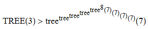
Theorem 1: TREE(3) > f^5(8), where f(n) := tree^n(7)
To prove this (see here for definitions), it is sufficient to exhibit a sequence of trees whose nodes are each coloured red, green, or blue, such that there is no colour-preserving embedding of an earlier tree into a later tree. We begin the sequence as follows:
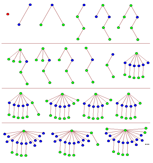
The first tree is a single red node, and we henceforth have no red nodes in any of the later trees. The twelfth tree, T12, and all subsequent trees have a single green root node connected to:
- n branches containing a single blue node attached to a single green leaf;
- m branches containing a single blue leaf;
- one or more green trees.
Trees T1 through to T11 can be seen to not embed into any tree of this form, so it remains to define the sequence {T12, ….} and show that none of these trees embeds into any later tree.
The sequence begins as follows:
T1 {}
T2 [[]]
T3 [()()]
T4 [((()))]
T5 ([(())][])
T6 ([(())](()))
T7 ([(())]()()())
T8 ([(())]()())
T9 ([(())]())
T10 ([(())])
T11 [(())]
T12 ([()][()][()][()][()][])
T13 ([()][()][()][()][()](()))
T14 ([()][()][()][()][()]()()())
T15 ([()][()][()][()][()]()())
T16 ([()][()][()][()][()]())
T17 ([()][()][()][()][()])
T18 ([()][()][()][()][][][][][][][][][])
T19 ([()][()][()][()][][][][][][][][](()))
T20 ([()][()][()][()][][][][][][][][]()()())
T21 ([()][()][()][()][][][][][][][][]()())
T22 ([()][()][()][()][][][][][][][][]())
T23 ([()][()][()][()][][][][][][][][])
T24 ([()][()][()][()][][][][][][][]X7)
where X7 is any (monochromatically green) tree on 7 vertices. This can be followed by the sequence:
T25 ([()][()][()][()][][][][][][][]X8)
T26 ([()][()][()][()][][][][][][][]X9)
T27 ([()][()][()][()][][][][][][][]X10)
...
T_(23 + tree(7)) ([()][()][()][()][][][][][][][]())
where X7, X8, X9, X10, … () is a maximal-length sequence for tree(7). If any earlier tree here embeds into a later tree, then the same must have been true in the maximal-length sequence for tree(7), contradicting the definition.
Consequently, we’ve already proved that TREE(3) > tree(7). We can then extend the sequence further by ‘burning’ another blue node (pair of square brackets):
T_(24 + tree(7)) ([()][()][()][()][][][][][][][])
T_(25 + tree(7)) ([()][()][()][()][][][][][][]Y1)
where Y1 is the first tree in the maximal-length sequence for tree(tree(7)). We proceed in the same way as before with a sequence of tree(tree(7)) terms, culminating in:
T_(23 + tree(7) + tree(tree(7))) ([()][()][()][()][][][][][][]())
T_(24 + tree(7) + tree(tree(7))) ([()][()][()][()][][][][][][])
T_(25 + tree(7) + tree(tree(7))) ([()][()][()][()][][][][][]Y2)
where Y2 is the first tree in the maximal-length sequence for tree(tree(tree(7))). Repeating this process, we eventually reach the tree:
([()][()][()][()])
at time 24 + tree(7) + tree(tree(7)) + … + tree^8(7). We can then make the next tree in our process have the form:
([()][()][()][][][][][]...[]X7)
where we have created tree^8(7) new blue nodes by ‘burning’ a branch of the form [()]. The same argument as before allows us to reach the tree:
([()][()][()])
at time well beyond tree^(tree^8(7))(7). Repeating this outer iteration another three times gets us to the claimed bound.
To see that no tree embeds homeomorphically into a later tree, we note that if T precedes T’, then we have at least one of the following:
- T contains more copies of [()] than T’;
- T contains more copies of [] than T’;
- The monochromatic green subtree of T precedes (in some tree(k) sequence) the monochromatic green subtree of T’;
where the latter condition was ensured by using a sequence for tree(k) which has this property by definition.
Theorem 2: tree(n) outgrows f_alpha(n) for every alpha preceding the small Veblen ordinal
This is implied by the statement in Harvey Friedman’s e-mails to the FOM mailing list:
One of our many finite forms of Kruskal's theorem asserts that

for all k, TREE[k] exists.

This function eventually dominates every provably recursive
function of the system ACA_0 + Pi12-BI.
and this is elaborated upon in Deedlit’s excellent MathOverflow answer.
Theorem 3: SSCG(4n + 3) >= SCG(n)
Conveniently, someone had e-mailed me to ask for an explicit proof of this statement, so I’ll include the reply I sent:
Suppose you have a sequence of N = SCG(n) (not necessarily simple)
subcubic graphs, (G_1, ..., G_N), such that G_i has at most i + n
vertices and no graph is a minor of a later graph.

Now, we let H_i be obtained from G_i by replacing each vertex with
a copy of the 4-vertex 3-edge Y-shaped graph, K3,1. For each pair
of adjacent vertices in the original graph, we join two as-yet-unused
'limbs' of the corresponding Y-shapes in the new graph. Then H_i is
simple and subcubic, and we can show that no graph is a minor of a
later graph. This is most easily shown by the fact that for subcubic
graphs, 'minor' is equivalent to 'topological minor', so it suffices
to show that no graph is homeomorphically embeddable into a later
graph. (Proof: if H_i embeds into H_j, the degree-3 vertices of H_i
must map to degree-3 vertices of H_j; this induces a homeomorphic
embedding from G_i to G_j.)

At this point we're almost done. The graphs (H_1, H_2, H_3, ...)
have at most (4n + 4, 4n + 8, 4n + 12, ...) vertices, respectively.
To prove the claim, we actually want a sequence with at most
(4n + 4, 4n + 5, 4n + 6, ...).

Now, since G_1 contains at least 2 vertices, it must contain at
least 1 edge which is not a self-loop (otherwise, every vertex has
degree <= 2 and we can add another edge, producing a more optimal
initial graph G_0, contradicting the assumption that our original
sequence of graphs is maximal). Consequently, H_1 contains a path
of vertices of degrees (3, 2, 2, 3). Let H_1' be the graph obtained
by contracting this path once, and H_1'' be the graph obtained by
contracting it again. Then the graphs (H_1, H_1', H_1'', H_2, H_3,
...) have the property that no graph is a minor of a later graph.

Hence, we can construct the sequence which begins:

- H_1 with at most 4n + 4 vertices;
- (H_1' + K_2) with at most 4n + 5 vertices;
- (H_1' + K_1 + K_1) with at most 4n + 6 vertices;
- (H_1' + K_1) with at most 4n + 7 vertices;
- H_1' with at most 4n + 8 vertices;
- (H_1'' + C_7) with at most 4n + 9 vertices;
- (H_1'' + C_6) with at most 4n + 10 vertices;
- (H_1'' + C_5) with at most 4n + 11 vertices;

where + denotes disjoint union of graphs. At this point, we've
'bought ourselves enough vertices' to continue the sequence as
follows:

- (H_2 + K_1 + K_1 + K_1 + K_1) with at most 4n + 12 vertices;
- (H_2 + K_1 + K_1 + K_1) with at most 4n + 13 vertices;
- (H_2 + K_1 + K_1) with at most 4n + 14 vertices;
- (H_2 + K_1) with at most 4n + 15 vertices;

- (H_3 + K_1 + K_1 + K_1 + K_1) with at most 4n + 16 vertices;
- (H_3 + K_1 + K_1 + K_1) with at most 4n + 17 vertices;
- (H_3 + K_1 + K_1) with at most 4n + 18 vertices;
- (H_3 + K_1) with at most 4n + 19 vertices;

and so forth. The property of no graph being a minor of a later
graph can easily be seen to be true, because at each iteration
we either have:

 - the 'big component' (the union of connected components which
contain at least one degree-3 vertex) gets strictly smaller (in
the poset of graphs under the minorship relation);
 - or the 'big component' stays identical and the 'small
component' gets strictly smaller;

and any homeomorphic embedding of one graph into another must map
the big component of the first graph into the big component of the
other graph.

I'm sure that there's enough slack in this proof to improve the
upper bound to SSCG(4n + 2) (by starting with H_1' instead of H_1),
but this proof suffices to show the claimed statement.
Theorem 4: SSCG(3) > TREE^(TREE^2(3))(3)
Again, we want to exhibit a sequence for SSCG(3) which exceeds TREE^(TREE^2(3))(3). We can begin as follows:
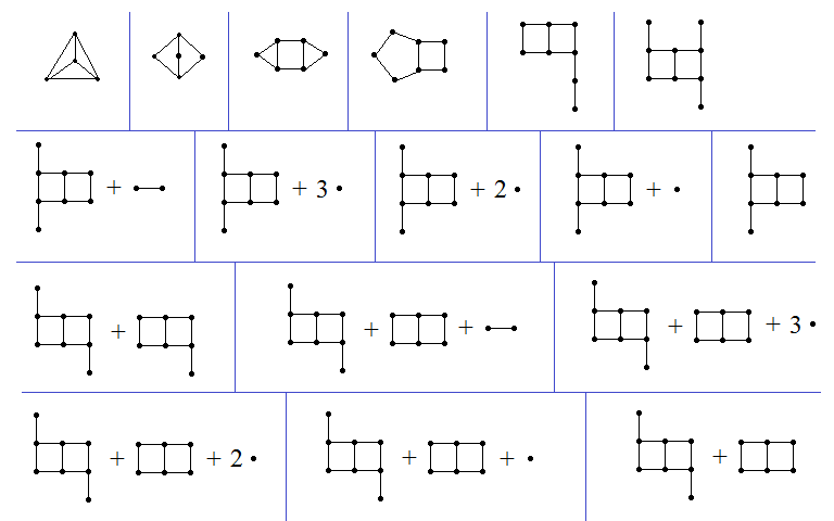
All subsequent graphs are the disjoint union of:
- p copies of the double-square with leaves attached to two diametrically opposite degree-2 vertices;
- q copies of the double-square with leaves attached to two degree-2 vertices which are neither adjacent nor diametrically opposite;
- r copies of the double-square with a single leaf;
- s copies of the double-square;
- a graph T which does not contain the double-square as a graph minor.
For example, the last graph in the above sequence is (1, 0, 0, 1, Ø), where Ø is the graph with no vertices or edges.
We define a sequence such that if the graph (p, q, r, s, T) precedes the graph (p’, q’, r’, s’, T’) in the sequence we define, then we have one of the following:
- p > p’;
- p = p’ and q > q’;
- (p, q) = (p’, q’) and r > r’;
- (p, q, r) = (p’, q’, r’) and s > s’;
- (p, q, r, s) = (p’, q’, r’, s’) and T is not a graph minor of T’.
With this convenient notation, we can write down some more terms of the sequence:
G18 (1, 0, 0, 0, 15-cycle)
G19 (1, 0, 0, 0, 14-cycle)
...
G29 (1, 0, 0, 0, square)
G30 (1, 0, 0, 0, triangle = H1)
G31 (1, 0, 0, 0, H2)
G32 (1, 0, 0, 0, H3)
...
G(2^(3 × 2^95) + 20) (1, 0, 0, 0, isolated_vertex)
G(2^(3 × 2^95) + 21) (1, 0, 0, 0, Ø)
where H1, H2, H3, … is the sequence of length 2^(3 × 2^95) − 9 that provides a lower bound for SSCG(2).
We can encode a rooted ordered coloured tree as a graph using the construction described here; this graph satisfies the properties required of T. The long initial segment of length 2^(3 × 2^95) + 21 means that we can use lots of vertices in the next step:
G(2^(3 × 2^95) + 22) (0, 2^(2^96), 0, 0, T1)
where T1 is the encoding of the first tree in a maximal-length sequence of rooted coloured trees for TREE(3). The ‘shrinking counter’ mechanism allows us to obtain a sequence of (l+7) TREE(3) graphs (none of which is a minor of any later graph) culminating in:
G(2^(3 × 2^95) + 22 + (l+7) TREE(3)) (0, 2^(2^96), 0, 0, Ø)
G(2^(3 × 2^95) + 23 + (l+7) TREE(3)) (0, 2^(2^96)-1, TREE(3), 0, U1)
where U1 is the encoding of the first tree in a maximal-length sequence of rooted coloured trees for TREE^2(3). At the end of the graph sequence corresponding to this tree sequence, we have the graph represented by the 5-tuple:
(0, 2^(2^96)-1, TREE(3), 0, Ø)
which can then be followed by:
(0, 2^(2^96)-1, TREE(3)-1, TREE^2(3), V1)
where V1 is the encoding of the first tree in a maximal-length sequence of rooted coloured trees for TREE^3(3). We can continue to repeat this same argument a total of TREE^2(3) times, decrementing the penultimate element of this 5-tuple each time, with the final iteration exceeding TREE^(TREE^2(3))(3) steps before we reach:
(0, 2^(2^96)-1, TREE(3)-1, 0, Ø)
This already proves what we set out to show, but it is clear that the iteration can go much further.

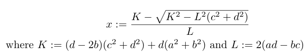
 is an integer.
 in both double-precision floating-point arithmetic (which is approximate) and in 64-bit integer arithmetic (which is exact, but reduced modulo 2^64).
 (n >= 3), whereas such a measure does exist in n = 2 dimensions as proved by Banach.
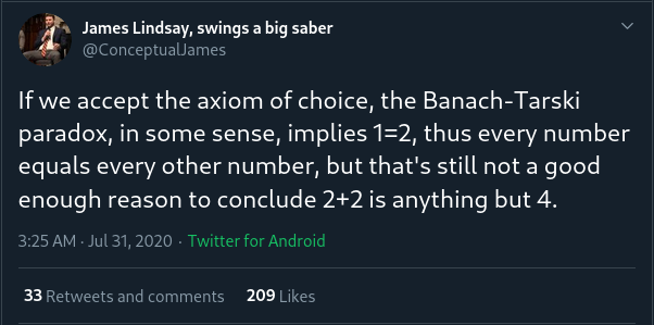
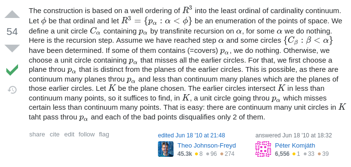
 is augmented with an extra point at infinity, where every pair of circles interlock in the same manner as these two rings of dodecahedra:
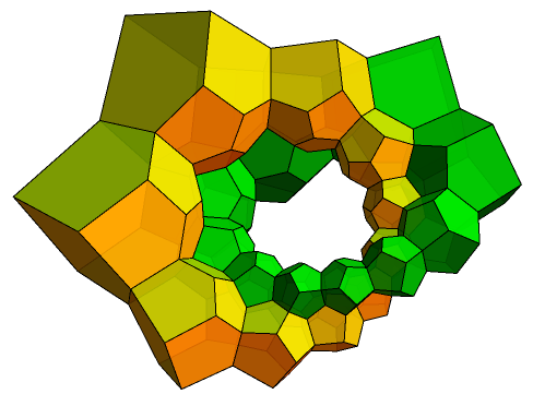
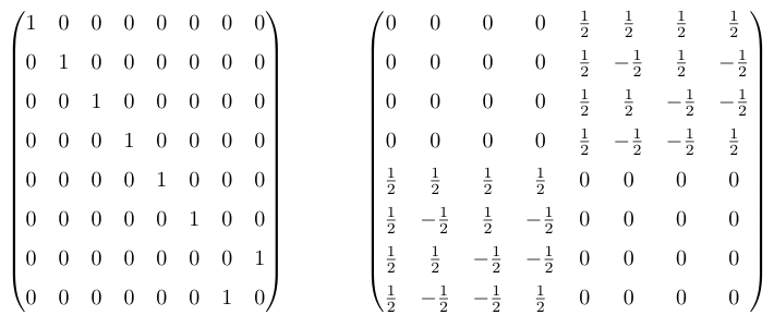
 . So, if
  is a unitary matrix, then all unitary matrices of the form
  induce the same transformation.
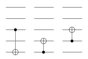
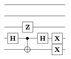
 , the CNOT gates induce linear shearing maps (and together generate the full 168-element group of linear automorphisms).
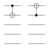
 (freely permuting the states 01, 10, and 11). These two gates, together with the three gates in the previous diagram, therefore generate the direct product
  of order 1008.
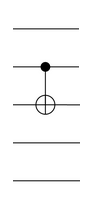
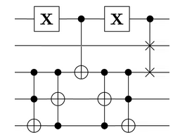
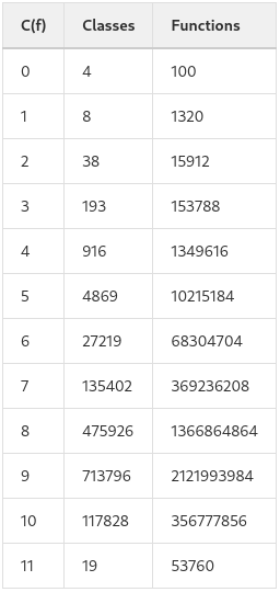
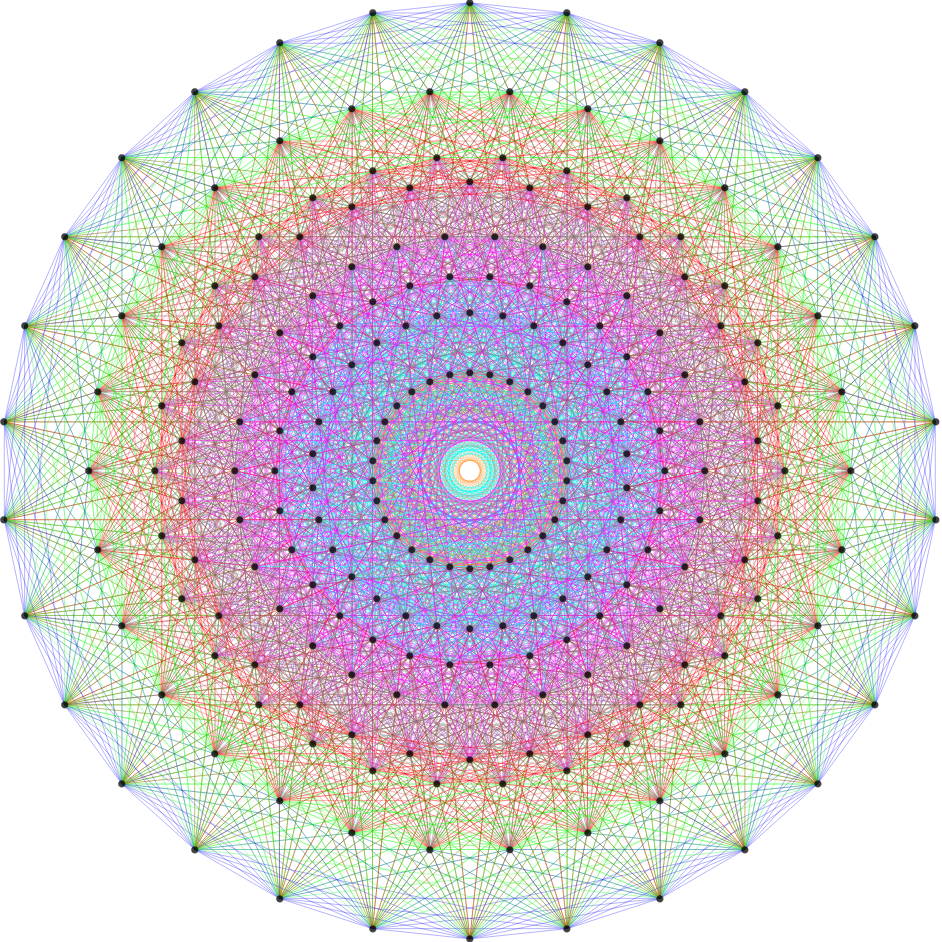
 qubits and the gates mentioned in the previous post, we remarked that the group generated is the full rotation group
  . If instead we replace the Toffoli gate in our arsenal with a CNOT gate, we get exactly the symmetry groups of the Barnes-Wall lattices! The orders of the groups are enumerated in
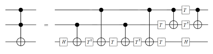
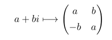
![\mathbb{Z}[\frac{1}{2}, \zeta]](https://s0.wp.com/latex.php?latex=%5Cmathbb%7BZ%7D%5B%5Cfrac%7B1%7D%7B2%7D%2C+%5Czeta%5D&bg=ffffff&fg=000&s=0&c=20201002) where ζ is a primitive eighth root of unity. A similar trick means we can work over the ring of dyadic rationals instead, at the cost of just two extra qubits:
where ζ is a primitive eighth root of unity. A similar trick means we can work over the ring of dyadic rationals instead, at the cost of just two extra qubits: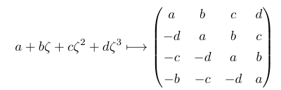