Complex Projective 4-Space

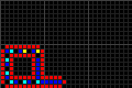
A new form of artificial life has been born — and there are no doubts that it directs its own self-replication:

So, what exactly is happening?

• At 0:06, the organism begins to sequentially construct four identical copies of itself.
• At 0:14, the original organism self-destructs to leave room for its offspring.
• At 0:16, each of the four children begin to sequentially construct copies of themselves. By 0:18, there are eight organisms.
• By 0:24, there are a total of thirteen organisms.
• At 0:27, the four from the previous generation self-destruct, followed shortly by the eight outermost organisms.
• By 0:34, the apoptosis of the outermost organisms finishes, leaving behind a clean isolated copy indistinguishable from the original cell.

How does it work? Why did the cells suddenly choose to die, and how did the middle cell know that it was due to survive? And how does this relate to multicellular life?

Update, 2019-05-12: Here’s a high-definition video of the construction of the south-east daughter machine:

History

The field of artificial life is often ascribed to Christopher Langton’s self-replicating loops. We have discussed these previously. A sequence of simple LOGO-like instructions circulate in an ensheathed loop. This information is executed 4 times to construct another copy of the loop (taking advantage of the symmetry of the daughter loop), and then the same tape is copied into the daughter loop:

Langton’s loop

If we quantify the number of times the loop’s instruction tape is utilised, we can represent it as the formal sum 4E + 1C (where ‘E’ represents one tape execution and ‘C’ represents tape copying).

However, there’s more. If the loop were only able to produce one child, the number of fertile loops would remain bounded (at 1), and it is disputed whether such bounded-fecundity ‘linear propagators‘ are actually true self-replicators. Note that at the end of the animation above, the loop has extended a new pseudopodium upwards, and will begin constructing a second offspring.

This continues for each of the sides of the parent loop, thereby giving an overall tape utility of 4(4E + 1C) = 16E + 4C. Note that the inner ‘4E’ comes from the fourfold symmetry of the daughter loop, whereas the outer ‘4E’ comes from the fourfold symmetry of the parent loop.

Anyway, after a while, the colony of self-replicating loops resemble this:

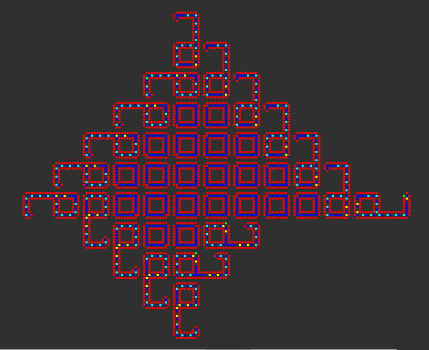
Colony of Langton’s self-replicating loops. The number of fertile loops grows linearly without bound, and the total number of loops (including the necrotic core at the centre) grows quadratically as a function of time.

Race to the bottom

Five years after Langton’s loops were invented, John Byl removed the inner sheath of the loop to result in a more minimalistic self-replicator, with only 4 tape cells surrounded by 8 sheath cells:

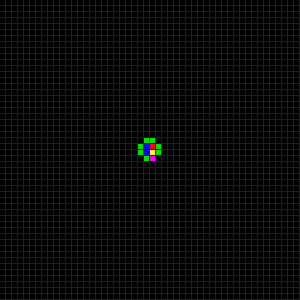
Byl’s simpler self-replicating loop. Image courtesy of Claudio Rocchini

Moreover, the underlying rule is simpler: only 6 states instead of 8. This comes at the expense of reduced flexibility; whereas one could build a larger Langton’s loop by increasing each side-length by n and inserting n ‘move forward’ instructions into the loop, there is no way to construct a Byl loop with any other genome.

Nor does it stop with Byl. In 1993, Chou and Reggia removed the outer sheath from the loop by adding two more states (returning to 8, same as Langton). The loops, which are barely recognisable as such, are only 6 cells in size: half of Byl’s loop and an order of magnitude smaller than Langton’s.

If minimality were the only concern, all of these examples would be blown out of the water by Edward Fredkin’s single-cell replicator in the 2-state XOR rule. However, every configuration in that rule replicates, including a photograph of Fredkin, so it is hard to claim that this is self-directed.

Ancestors of Langton’s Loops

The inspiration for Langton’s loop was an earlier (1968) 8-state cellular automaton by E. F. Codd (the inventor of the relational database). Codd’s cellular automaton was designed to support universal computers augmented with universal construction capabilities: unlike Langton’s loops, the instruction tape can program the machine to build any configuration of quiescent cells, not just a simple copy of itself.

It took until 2010 before Codd’s machine was actually built, with some slight corrections, by Tim Hutton. It is massive:

Tim Hutton’s implementation of Codd’s self-replicating computer

Codd’s cellular automaton itself was borne out of a bet in a pub, where Codd challenged a friend that he could create a self-replicating computer in a cellular automaton with fewer states than von Neumann’s original 29-state cellular automaton.

Comparison of replicators

For an n-state k-neighbour cellular automaton, there are different rules, where is the number of distinct neighbourhoods that can occur. (We get equality in the case of asymmetric rules, but for rules with symmetries the count is more complex and depends on the Polya Enumeration Theorem.) Consequently, we can concretely define the ‘complexity’ of the rule (in bits) to be .

For instance, Langton’s, Codd’s and Chou-Reggia’s cellular automata all have a complexity of 25056 bits, whereas Nobili’s 32-state adaptation of von Neumann’s original 29-state rule has a complexity of 167772160 bits. Conway’s two-state rule, by comparison, has only 18 bits of complexity.

We can plot the population count (including the tape) of different self-replicating machines on one axis, and the complexity of the rule on the other axis. Interestingly, qualitative categories of replicator such as ‘universal constructor’, ‘loop’, and ‘parity-rule replicator’ form visually distinct clusters in the space:

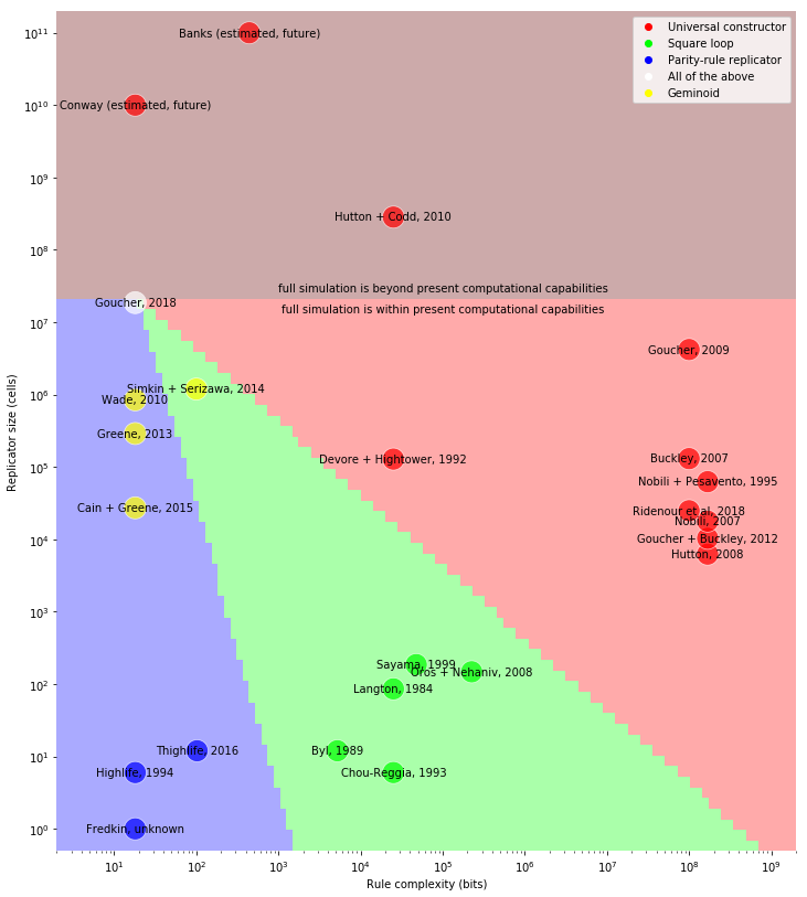
Near the top of the plot are two rough hypothetical designs of replicators which have never been built:

• Conway’s original blueprint for a universal constructor in his 2-state 9-neighbour cellular automaton, as described in Winning Ways and The Recursive Universe;
• An estimate of how large a self-replicating machine would need to be in Edwin Roger Banks’ ‘Banks-IV‘ cellular automaton, described in his 1971 PhD thesis.

The third point from the top (Codd’s 1968 self-replicating computer) also fell into this category, until Tim Hutton actually constructed the behemoth. This has been estimated to take 1000 years to replicate, which is why it is firmly above the threshold of ‘full simulation is beyond present computational capabilities’.

Everything else in this plot has been explicitly built and simulated for at least one full cycle of replication. Immediately below Codd’s machine, for instance, is Devore’s machine (built by Hightower in 1992), which is much more efficient and can be simulated within a reasonable time. The other patterns form clusters in the plot:

• On the right-hand side of the plot is a cluster of self-replicating machines in von Neumann cellular automata, along with Renato Nobili’s and Tim Hutton’s modifications of the rule.
• The green points in this centre at the bottom are loop-like replicators. As well as Langton’s loops, this includes evolvable variants by Sayama and Oros + Nehaniv.
• The bottom-left cluster comprises trivial parity-rule replicators which have no tape and are passively copied by the underlying rule.

The yellow points on the left edge are self-propagating configurations which move by universal construction, but are not replicators in the strictest sense. They are all bounded-fecundity self-constructors, and with the exception of Greene 2013, they do not even copy their own tapes.

Why is the new organism interesting?

Finally, we have the new organism (shown in white on the left-hand side of the log-log plot, immediately below the threshold of practicality). Suitably programmed, this is a parity-rule replicator, and a loop-like replicator, and a universal constructor. It is also the first unbounded-fecundity replicator in Conway’s 2-state cellular automaton.

If we look again at the video:

we can see that, macroscopically, it copies itself in all four directions similar to Langton’s loops. The circuitry is designed such that each new child is placed in the same orientation and phase as the parent. Moreover, we see that the organism is programmed to self-destruct — either before or after constructing up to four children.

Whether or not it self-destructs prematurely depends on what signals it has received from its neighbours. Effectively, the machine receives a signal (a positive integer between 1 and 7, inclusive) from each of the (up to four) neighbours, and a 0 from any empty spaces if there are fewer than four neighbours. It then computes the quantity , where (a, b, c, d) are the four input signals, and indexes into a 4096-element lookup table to retrieve a value between 0 and 7 (the new ‘state’ of the machine). If 0, it immediately self-destructs without constructing any children; if nonzero, it constructs a daughter machine in each vacant space. Finally, it broadcasts the new state as a signal to all four neighbours, before self-destructing anyway.

In doing so, this loop-like replicator behaves as a single cell in any 8-state 4-neighbour cellular automaton; the rule is specified by the lookup table inside the replicator. We call this construct a metacell because it emulates a single cell in a (8-state 4-neighbour) cellular automaton using a large collection of cells in the underlying (2-state 9-neighbour) cellular automaton.

This is not the first metacell (David Bell’s Unit Life Cell being the first example), but it is unique in having a 0-population ground state. As such, unlike the Unit Life Cell (which requires the entire plane to be tiled with infinitely many copies), any finite pattern in the emulated rule can be realised as a finite pattern in the underlying rule.

Interestingly, every 2-state 9-neighbour cellular automaton can be emulated at half the speed as an 8-state 4-neighbour cellular automaton. As such, we can ‘import’ any pattern from any such cellular automaton into Conway’s rule, thereby obtaining the first examples of:

• a parity-rule replicator (by emulating Fredkin, HighLife, or ThighLife);
• a reflectorless rotating oscillator;
• a spaceship made of perpetually colliding copies of smaller spaceships;

or even the metacell itself, recursively, obtaining an infinite sequence of exponentially larger and slower copies thereof (as if the existing metacell isn’t already too large and slow!).

To simplify the process of ‘metafying’ a pattern from an arbitrary isotropic 2-state 9-neighbour cellular automaton, I have included a Python script; this programs the metacell for the desired rule and assembles many copies (one for each cell in the original pattern) thereof into an equivalent pattern ‘writ large’.

Next time, we shall discuss in greater detail how the metacell itself was built. Until then, you may want to read Dave Greene’s recent article about some of the technology involved.

At the Heidelberg Laureate Forum three years ago, I took lots of selfies with Fields medallists, Abel prizewinners and Turing laureates. This included having a dinner in a castle with Leonard Adleman, pioneer of asymmetric cryptography:

…and Endre Szemeredi of regularity lemma fame…

…and Louis Nirenberg…

…and, last but certainly not least, enjoyed sparkling Riesling in a Bavarian brewery with Michael Atiyah:

He proceeded to summon several of us into a room, wherein he posed a rather interesting problem and offered a reward for its solution:

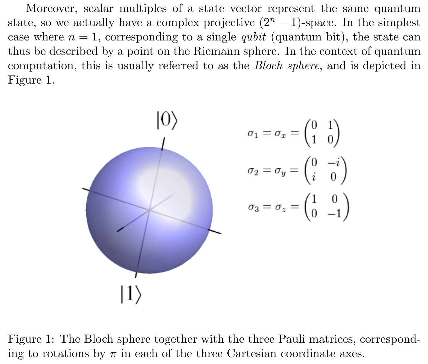
Consider n distinct points, in the three-dimensional unit ball. Let the ray (half-line) from through meet the boundary of the ball at , viewed as a complex number on the Riemann sphere. We define the monic polynomials whose roots are given by the projections of the remaining points onto the sphere.

Prove that these n polynomials are linearly independent.

If we consider the determinant of the matrix M formed by the coefficients of these polynomials, we get a degree-½n(n−1) homogeneous polynomial in the n(n−1) roots. This determinant can be seen to be invariant under adding a constant to all roots, but it is not scale-invariant because the degree is nonzero. This can be amended by dividing by a normalising constant, yielding a rational function δ:

Note that δ is not only scale- and translation-invariant, but also is invariant under simultaneously replacing all roots by their reciprocals. This means that δ is invariant under the entirety of the Möbius group, which corresponds naturally to the group of orientation-preserving projective transformations fixing the unit ball. Since δ is dimensionless, it is reasonable to conjecture the following stronger problem:

Prove that |δ| ≥ 1.

Apparently an acquaintance of Atiyah proved this for up to 4 points by symbolic manipulation in a computer algebra package, and experimentally verified that it appears to hold in much higher dimensions.

Interestingly, if one of the points is on the boundary of the unit ball, it can be seen that deleting it does not alter the value of δ. (Hint: since we have so much invariance, it suffices to check this at the point 0.) This allowed Atiyah to strengthen the problem even further:

Prove that, if we leave the points in-place and gradually shrink the ball until one of the points lies on the boundary, the value |δ| does not increase.

Atiyah circulated this problem to as many mathematicians as he could, offering a bottle of champagne and an invitation to the next HLF as a reward for anyone who could solve it. I was perplexed that Atiyah — who is a ‘theory-builder’ rather than a ‘problem-solver’ (e.g. Erdös) — would be interested in a problem that, whilst being elegant, seemingly bears no connection to serious research mathematics. I wondered whether he was following in the footsteps of Littlewood, who used to take disguised versions of the Riemann hypothesis and give them to PhD students as research problems.

Of course, I didn’t know at the time which great problem Atiyah had reduced to this lemma. Last year, however, he gave a talk at Cambridge presenting a proof of this geometrical inequality. I wasn’t at the talk, but apparently it involved expressing the logarithm of |δ| (possibly negated) as the von Neumann entropy of some system, and proving the strongest version of the conjecture as a corollary of entropy being non-decreasing.

On Monday morning, however, Atiyah will be presenting a proof of the Riemann hypothesis in a 45-minute talk at the Heidelberg Laureate Forum, three years after he presented this problem to us. The abstract of the forthcoming talk mentions that it builds upon work by von Neumann, which is tantalisingly consistent with my prediction that his ‘points in a ball’ conjecture was merely the remaining lemma required to solve a huge unsolved problem!

Anyway, in 60 hours’ time, number theory will be revolutionised. Let’s hope that his proof generalises easily to GRH as well, so that we can enjoy a deterministic primality test faster than AKS.

Important note: whenever log is mentioned in this particular post, it is referring to the ceiling of the base-2 (binary) logarithm. (Elsewhere on cp4space, when there isn’t this disclaimer, it refers to the base-e (natural) logarithm.)

For reasons that shall soon become clear, I found myself faced with the task of sorting a list of 12 objects.

Usually one would choose an algorithm such as quicksort or Timsort. Conventional comparison-based sorting algorithms operate by comparing pairs of objects, and are otherwise unrestricted: the choices of objects to compare can depend on the results of previous comparisons.

A sorting network is a much more restricted sorting algorithm, where the only allowed operation is the compare-exchange instruction CMPX(i, j). This compares objects in positions i and j, swapping them if they are in the wrong order, and revealing no information. Here are the best known sorting networks on 9 and 12 elements, photographed from The Art of Computer Programming by Donald Knuth:

So, with straight-line code of 39 CMPX instructions it is possible to sort a collection of 12 objects without any need for loops, conditional branching, or any other form of control flow. This is especially useful when programming a GPU, where control flow is toxic for performance.

I proceeded to transcribe the sorting network from the above diagram into CUDA code. As a mere mortal, I was not totally convinced that I’d copied it flawlessly, so resorted to building a test to verify the correctness of the transcribed network. Preferring to do this in a high-level language such as Python, I resorted to my usual tricks of writing a single file which is valid in two languages and incorporating it into the source code by means of one innocuous line: #include “sorting_network.py”

(If you think this is bad, people have done much worse…)

Examining the Python component of the code, you may notice that it only tests the 2^12 different binary sequences, rather than the 12! different totally ordered sets. It is a general property of comparator networks that it suffices to only test binary sequences to prove that the network can sort arbitrary sequences; this is known as the 0-1 principle.

Batcher’s bitonic mergesort

What is the minimum number of CMPX gates necessary to sort n objects? And what is the minimum circuit depth? The naive algorithm of bubble sort shows that a gate-count of O(n^2) and a circuit depth of O(n) are both attainable. Similarly, the gate-count must be at least the binary logarithm of n! (as with any comparison-based sorting algorithm) which gives a lower bound of Ω(n log n) for the gate-count and Ω(log n) for the depth.

Batcher found a recursive construction of sorting networks with a depth of ½k(k+1), where k is the ceiling of the binary logarithm of n, and each layer has ½n comparators. This is achieved by firstly Batcher-sorting the initial and final halves of the sequence, followed by interleaving them (diagram by User:Bitonic from Wikipedia):

The correctness of the algorithm follows from the aforementioned 0-1 principle. By the inductive hypothesis, it suffices to examine the rightmost blue box and suppose that the two halves of the input are correctly sorted, in which case the input would resemble:

[n/2 – m zeroes] [m ones] | [l zeroes] [n/2 – l ones]

The only ‘cross-lane’ operations are the comparators in the brown box. If l is no greater than m, the result of this is the following:

[n/2 – m zeroes] [m – l ones] [l zeroes] | [n/2 ones]

and otherwise we get the complementary arrangement:

[n/2 zeroes] | [m ones] [l – m zeroes] [n/2 – l ones]

Concentrating only on the non-constant half, our task is reduced to the simpler problem of sorting a binary sequence which switches at most twice between a run of zeroes and a run of ones. We can split the effect of the pink box into two modules: one which reverses one of the two halves (we get to decide which half!), followed by one which behaves identically to a brown box. Observe that, as before, one of the two halves of the pink box must therefore be constant, and the other must again be a binary sequence which switches at most twice. By induction, the result follows.

Owing to the low depth, simplicity, and efficiency, Batcher’s bitonic mergesort is often used for sorting large lists on GPUs.

Beyond Batcher

But is the bitonic mergesort optimal? The circuit above takes 80 comparators to sort 16 inputs, whereas the best circuit in Knuth takes only 60 comparators (again with a depth of 10). It’s not even optimal for depth, as the next page of Knuth has a 61-comparator sorting network with a depth of 9.

What about asymptotics? The bitonic mergesort gives an upper bound on the depth of O((log n)^2) and basic information theory gives a lower bound of Ω(log n).

The next surprise was when Szemeredi, Komlos and Ajtai proved that the lower bound is tight: they exhibited a construction of sorting networks of optimal depth O(log n). As you can imagine from Szemeredi’s background in combinatorics and extremal graph theory, the construction relies on a family of graphs called expanders.

A simplified version of the construction (by Paterson, 1990) is described here. The original paper provides explicit constants, showing that a depth ~ 6100 log(n) is possible, compared with ~ ½ log(n)^2 for Batcher’s bitonic mergesort. In other words, the threshold for switching from bitonic mergesort to Paterson’s variant of AKS occurs when n is approximately 2^12200.

A further improvement by Chvatal reduces the asymptotic constant from 6100 to 1830, and actually provides an explicit (non-asymptotic) bound: provided n ≥ 2^78, there is a sorting network of depth 1830 log(n) − 58657. This reduces the crossover point to exactly n ≥ 2^3627. As Knuth remarked, this is still far greater than the number of atoms in the observable universe, so the practical utility of the AKS sorting algorithm is questionable.

Interestingly, this is not the first time there has been an asymptotically impressive algorithm named AKS after its authors: a set of three Indian Institute of Technology undergraduates {Agrawal, Kayal, Saxena} found the first unconditional deterministic polynomial-time algorithm for testing whether an n-digit number is prime. This O(n^(6+o(1)) algorithm tends not to be used in practice, because everyone believes the Generalised Riemann Hypothesis and its implication that the O(n^(4+o(1)) deterministic Miller-Rabin algorithm is correct.

Congratulations to Meghan Markle and Prince Harry on what is undoubtedly the most energetic Royal Wedding!

In other news, following on from Aubrey de Grey’s 5-chromatic unit-distance graph, there has been an effort to study the algebraic structure of the graphs. Specifically, viewing the vertices as points in the complex plane, one can ask what number fields contain the vertices of the unit-distance graphs.

In particular, it was noted that both Moser’s spindle and Golomb’s graph, the smallest examples of 4-chromatic unit-distance graphs, lie in the ring , where is a complex number with real part and absolute value 1. Ed Pegg Jr produced a beautiful demonstration of this:

Philip Gibbs showed that the entire ring, and consequently all graphs therein, can be coloured by a homomorphism to a four-element group. Consequently, Ed Pegg’s hope that the large unit-distance graph above is 5-chromatic was doomed to fail — but that is not too much of a worry now that we have de Grey’s 5-chromatic graph.

Several of Marijn Heule’s 5-chromatic graphs lie in . Apparently both this ring and have homomorphic 5-colourings, so we cannot find a 6-chromatic unit-distance graph lying in either of these rings.

Incidentally, the record is a 610-vertex example, again due to Heule: