Congratulations to Meghan Markle and Prince Harry on what is undoubtedly the most energetic Royal Wedding!
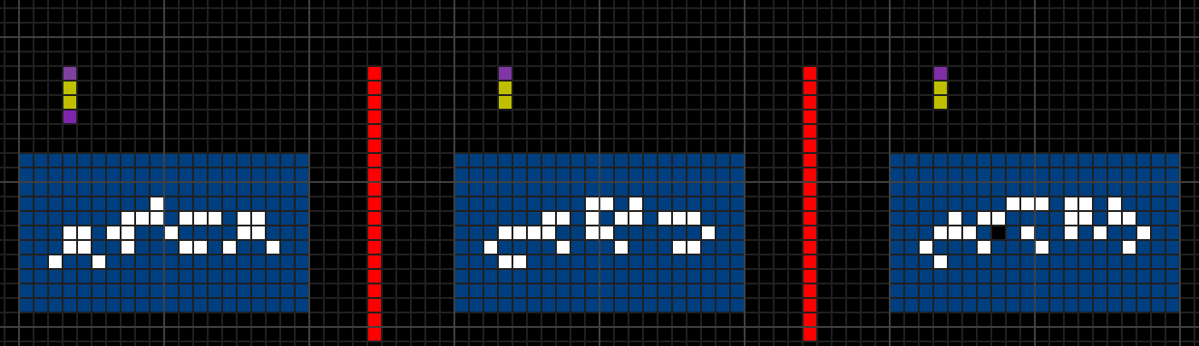
In other news, following on from Aubrey de Grey’s 5-chromatic unit-distance graph, there has been an effort to study the algebraic structure of the graphs. Specifically, viewing the vertices as points in the complex plane, one can ask what number fields contain the vertices of the unit-distance graphs.
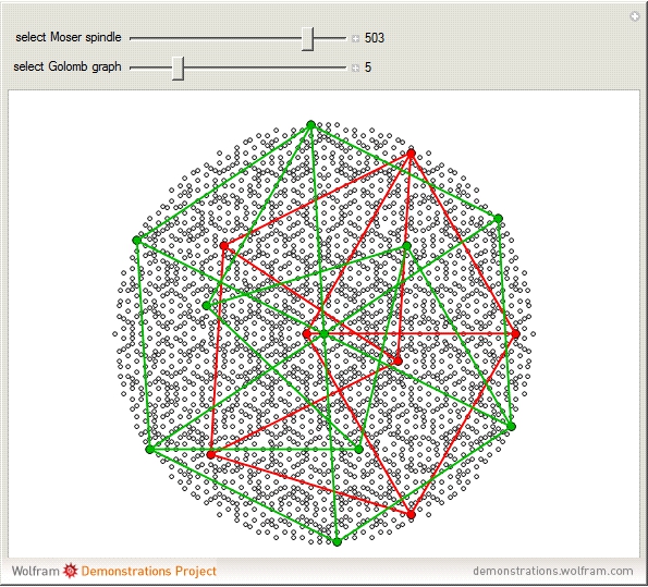
In particular, it was noted that both Moser’s spindle and Golomb’s graph, the smallest examples of 4-chromatic unit-distance graphs, lie in the ring , where is a complex number with real part and absolute value 1. Ed Pegg Jr produced a beautiful demonstration of this:
Philip Gibbs showed that the entire ring, and consequently all graphs therein, can be coloured by a homomorphism to a four-element group. Consequently, Ed Pegg’s hope that the large unit-distance graph above is 5-chromatic was doomed to fail — but that is not too much of a worry now that we have de Grey’s 5-chromatic graph.
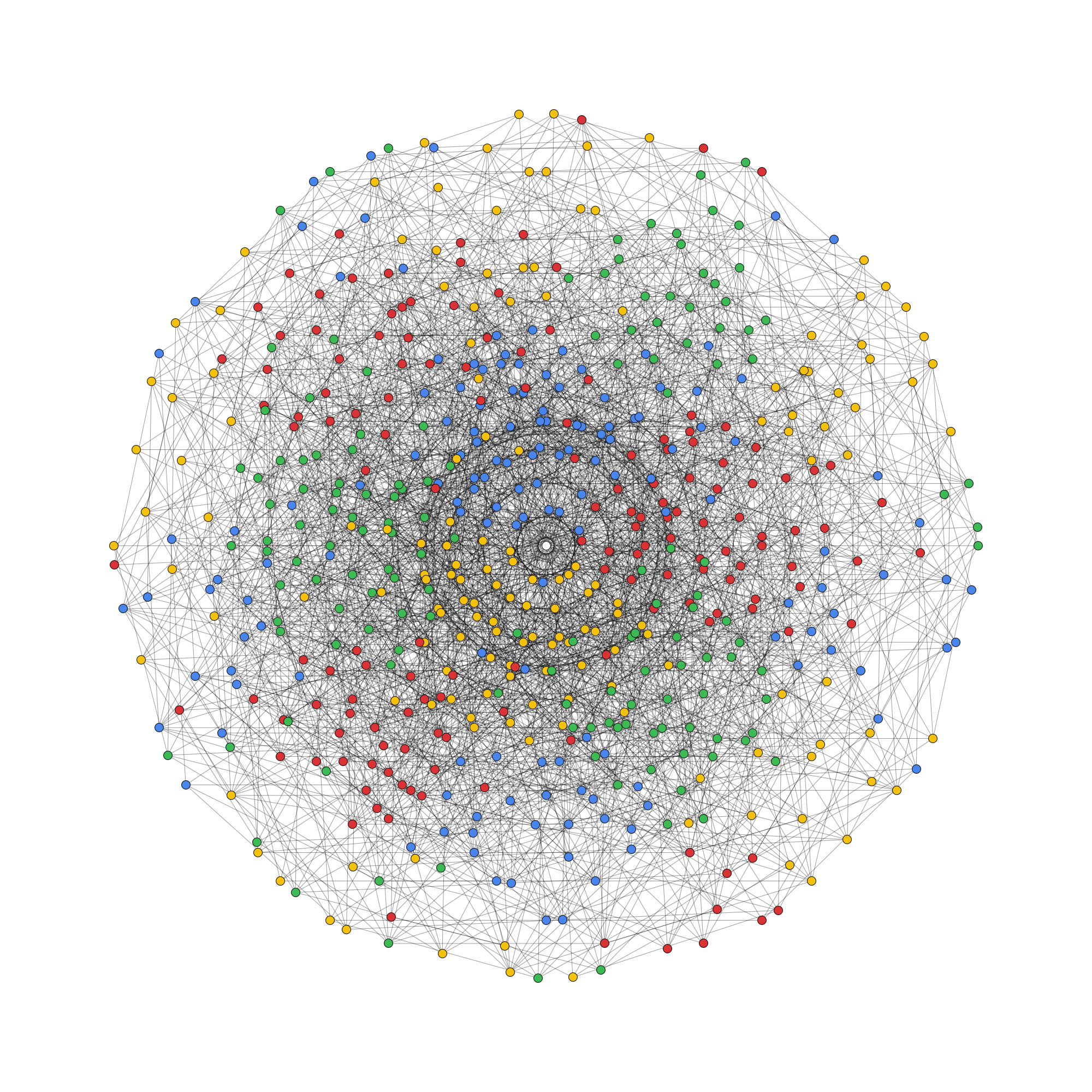
Several of Marijn Heule’s 5-chromatic graphs lie in . Apparently both this ring and have homomorphic 5-colourings, so we cannot find a 6-chromatic unit-distance graph lying in either of these rings.
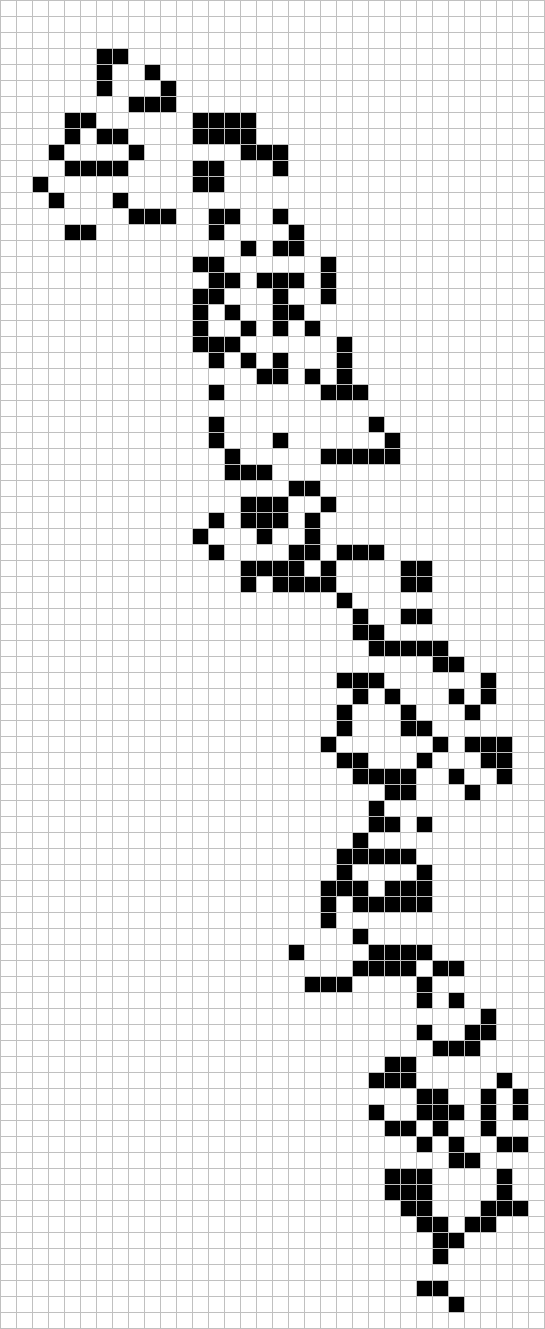
Incidentally, the record is a 610-vertex example, again due to Heule:
This last week has been very exciting. On Thursday, I gave a talk in absentia at the 13th Gathering for Gardner on the topic of artificial life (thanks go to Dave Greene and Tom Rokicki for playing the slides and audio recording). Meanwhile, this happened:
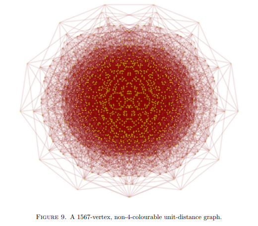
Chromatic number of the plane is at least 5
Aubrey de Grey (!!!) has found a unit-distance graph with 1567 vertices and a chromatic number of 5. This implies that the chromatic number of the plane is between 5 and 7, the latter bound obtainable from 7-colouring the cells of an appropriately-sized hexagonal lattice. Before, the best lower bound was 4 (from the Moser spindle).
There is now a polymath project to reduce the number of vertices from 1567. Marijn Heule, whom I mentioned last time for providing me with the incremental SAT solver used to find Sir Robin, has already reduced it down to 874 vertices and 4461 edges.
EGMO results
The results of the European Girls’ Mathematical Olympiad have been published. The UK came third worldwide, just behind Russia and the USA. Moreover, Emily Beatty was one of five contestants to gain all of the available marks, and apparently the first UK contestant to do so in any international mathematical competition since 1994.
It appears that EGMO has been following the example of the Eurovision Song Contest in determining which countries are European, rather than actually verifying this by looking at a map. Interesting additions include the USA, Canada, Saudi Arabia, Israel, Australia, Mongolia, Mexico and Brazil. The list of participating countries states that there are 52 teams, of which 36 are officially European (and a smaller number still are in the EU).
Restricting to the set of countries in the European Union, the UK won outright (three points ahead of Poland), which was the last opportunity to do so before the end of the Article 50 negotiations. Hungary and Romania put in a very strong performance, as expected.
Previously, we discussed Homotopy Type Theory, which is an alternative foundation of mathematics with several advantages over ZFC, mainly for computer-assisted proofs. It is based on Martin-Löf’s intuitionistic type theory, but with the idea that types are spaces, terms are points within that space, and that A = B is the space of paths between A and B (viewed as points in a universe U). To accomplish this, recall that there are two extra modifications beyond intuitionistic type theory:
Voevodsky’s univalence axiom states that equivalent types are equal, and more specifically that the space of equivalences between two types is equivalent to the space of paths between two types;
The introduction of higher inductive types which define not only their elements (vertices) but also paths, 2-cells (paths between paths), and so forth.
An advantage of intuitionistic type theory is that the lack of axioms mean that all proofs of constructive. Including the univalence axiom breaks this somewhat, which is why people have been searching for a way to adapt type theory to admit univalence not as an axiom, but as a theorem.
Cubical type theory was introduced as a constructive formulation which includes univalence and has limited support for certain higher inductive types. A recent paper by Thierry Coquand (after whom the automated theorem-prover Coq is named), Simon Huber, and Anders Mörtberg goes further towards constructing higher inductive types in cubical type theory.
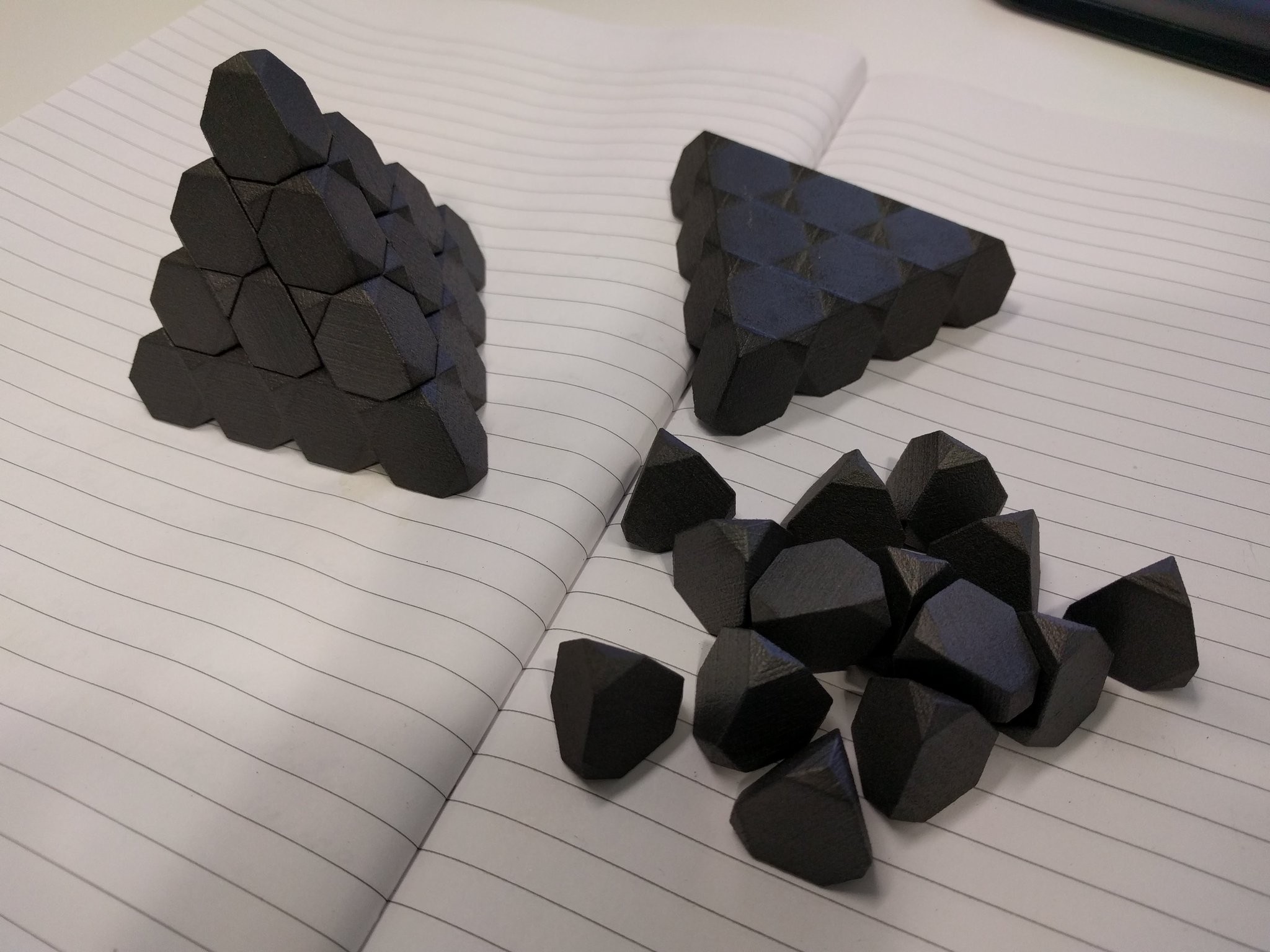
Tim Hutton recently presented me with a marvellous 3D-printed-graphite set of triakis truncated tetrahedra. These have a natural interpretation as the Voronoi cells of a diamond: the shapes that would form if you gradually enlarged the atoms until they tessellate the ambient space.
He also produced a video describing the relationship between the Voronoi cells of the diamond and related lattices.
Hyperdiamonds
Mathematically, the set of centres of atoms in a diamond form a structure called . It has a natural n-dimensional generalisation, which can be viewed as follows:
Take the integer lattice ;
Partition it into two subsets, called E and O, consisting of the points whose coordinate-sums are even and odd, respectively;
Translate the set O such that it contains the point (½, ½, ½, …, ½), and leave E where it is.
This construction makes it adamantly* clear that the ‘hyperdiamond’ has the same density as the integer lattice, and therefore the Voronoi cells have unit volume. A lattice with this property (such as the hyperdiamonds of even dimension) is described as unimodular.
*bizarrely, this word has the same etymology as ‘diamond’, namely the Greek word adamas meaning ‘indestructible’. I often enjoy claiming that my own given name is also derived from this same etymology.
In the special case where n = 8, this is the remarkable E8 lattice, which Maryna Viazovska proved is the densest way to pack spheres in eight-dimensional space. One could imagine that if beings existed in eight-dimensional space, they would have very heavy diamond engagement rings! It is an even unimodular lattice, meaning that the inner product of any two vectors is an even integer, and is the unique such lattice in eight dimensions. They can only exist in dimensions divisible by 8, and are enumerated in A054909.
If n = 16, the hyperdiamond gives one of two even unimodular 16-dimensional lattices, the other being the Cartesian product of E8 with itself. These two lattices have the same theta series (sequence giving the number of points at each distance from the origin), but are nonetheless distinct. If you take the quotients of 16-dimensional space by each of these two lattices, you get two very similar (but non-isometric) tori which Milnor gave as a solution to the question of whether two differently-shaped drums could produce the same sound when reverberated.
John Baez elaborates on the sequence of ‘hyperdiamonds’, together with mentioning an alternative three-dimensional structure called the triamond, here.
Niemeier lattices
There are 24 even unimodular lattices in 24 dimensions, the so-called Niemeier lattices, of which the most famous and stunning is the Leech lattice. This was also proved by Viazovska and collaborators to be the densest sphere packing in its dimension. Unlike the hyperdiamonds, however, the Leech lattice is remarkably complicated to construct.
Whereas the shortest nonzero vectors in the Leech lattice have squared norm of 4, the other 23 Niemeier lattices have roots (elements of squared norm 2). The Dynkin diagrams of these root systems identify the lattices uniquely, and conversely all Dynkin diagrams with certain properties give rise to Niemeier lattices.
The 23 other Niemeier lattices correspond exactly to the equivalence classes of deep holes in the Leech lattice, points at a maximum distance from any of the lattice points.
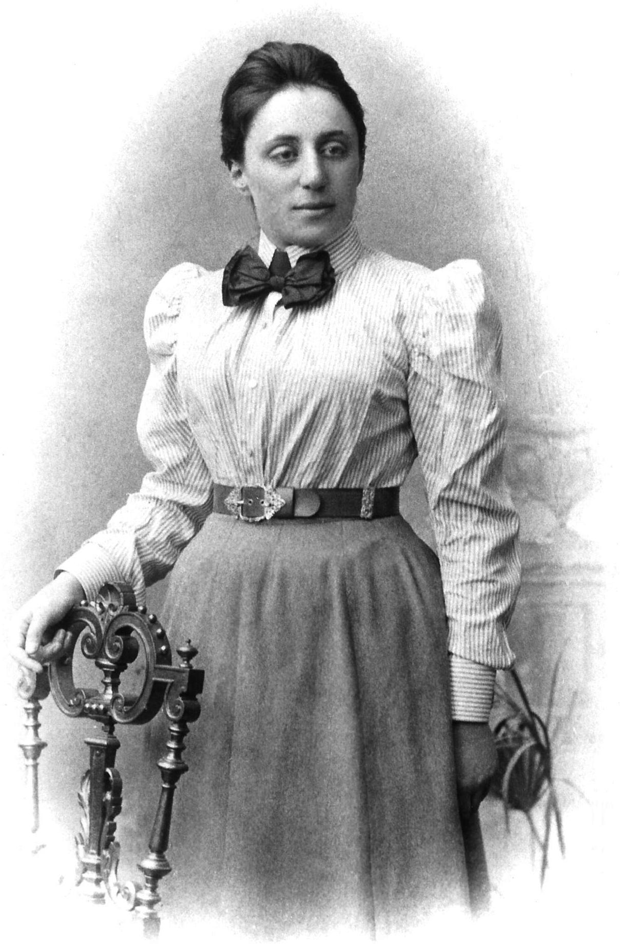
I’ve just realised, with only two minutes to go, that it’s the 136th birthday of the great mathematician Emmy Noether.
Naturally, you are probably already aware of many of her contributions to mathematics and theoretical physics, including Noetherian rings and Noether’s theorem. I was pleasantly surprised to hear that she also laid the foundations of homology theory, which is especially pertinent as my research in topological data analysis is built upon these ideas.
Conway and Sloane’s excellent tome, Sphere Packings, Lattices and Groups, is now due a fourth edition. Maryna Viakovska’s proofs of optimality of the E8 and Leech lattices should go in the fourth edition as well…
Over the last couple of months, I have been experimenting with the use of SAT solvers. This research recently came to fruition, with Tomas Rokicki and me announcing a new discovery with the intention of writing up the methodology in a paper.
Academic papers, however, typically feature a polished proof which omits all of the insights and attempts and failures which led to its discovery. This post attempts to remedy that by presenting a chronological itemisation of the journey; the technical details will be largely reserved for the paper.
30th January: graph theory supervisions
The previous term I had been supervising a lecture course on Graph Theory for the university. One of the questions on the final example sheet was the following:
11. Let G be a graph in which every edge is in a unique triangle and every non-edge is a diagonal of a unique 4-cycle. Show that |G| ∈ {3, 9, 99, 243, 6273, 494019}.
The usual method of solving this problem is to show that the graph must be regular, and therefore strongly regular; the resulting finite set of possibilities drops out from considering the eigenvalues of the adjacency matrix and observing that their multiplicities must be integers.
It is interesting to ask whether there actually exist suitable graphs with these numbers of vertices. For 3 vertices, a triangle obviously works; for 9 vertices, the toroidal 3-by-3 grid graph is a solution. There is also a known example with 243 vertices, related to the remarkable ternary Golay code. For 99, 6273, or 494019 vertices, however, it is unknown whether there is such a graph.
I mentioned in the supervision that John Conway had offered $1000 for a resolution of whether the 99-vertex graph exists, still unclaimed. One of my supervisees asked whether it could be amenable to computer search, and I responded that it might be within reach of a SAT solver: an algorithm for determining whether a set of Boolean equations has a solution.
The 99-graph problem is of a similar size to the Boolean Pythagorean Triples Problem, recently defeated by Marijn Heule and an army of SAT solvers. The UNSAT certificate (proof generated by the machine) is 200 terabytes in length, making it the largest proof of any mathematical problem in history. (The 13-gigabyte Erdös discrepancy proof, also found by SAT solvers, pales in comparison!)
At this point, I thought I would have a go at attacking the 99-graph problem myself. I’d done roughly as much exploration of the necessary structure of the graph as could be accomplished within a single side of A4 paper, and felt it was in a form amenable to SAT solving. I read several academic papers about SAT solvers, and closely monitored the competition results, to reach the conclusion that the state-of-the-art technique for approaching large SAT problems proceeds along lines similar to the following:
Initially simplify the problem using lingeling -S;
Split the problem space using march-cc into thousands of separate ‘cubes’;
Share the cubes amongst parallel instances of the incremental SAT solver iglucose.
I started to develop a framework, which I called MetaSAT, for automating this process. Coincidentally, at the same time, someone else also became interested in SAT solvers…
26th January: Oscar Cunningham’s LLS
In his Odyssean epic The Art of Computer Programming, Donald Knuth dedicates a large section to SAT solvers with a particular emphasis on applying them to Conway’s Game of Life. This left the realms of theory and entered practice when Oscar Cunningham, who studied mathematics in Cambridge at roughly the same time as I did (and taught me how to play frisbee), wrote a Python script to search for patterns using Knuth’s ideas.
Logic Life Search, or LLS, is a sophisticated Python search program capable of using one of many different SAT solvers as backends to find patterns in various cellular automata.
This drove me to attempt to integrate these ideas into the MetaSAT project, so that I could search larger spaces than is possible with a single SAT solver. What I ended up doing was creating a simplified Golly-compatible version of LLS, called GRILLS. Whilst LLS is strictly more powerful, GRILLS has a more user-friendly graphical interface, and allows for loading results from previous runs:
I departed slightly from Donald Knuth’s binary-tree approach of counting neighbours, instead opting for a ‘split-radix’ binary-ternary tree. This reduced the number of variables needed by the SAT solver by 40%, without affecting the number of clauses, thereby making the problem slightly easier to digest (at least in principle).
The pinnacle of its success was being able to find an already-known c/4 orthogonal spaceship. Whilst showing that SAT solvers could replicate existing discoveries, there was no evidence that they could find anything new — in other words, they seemed to be trailing behind discoveries found with special-purpose CA search programs.
31st January: Tomas Rokicki’s c/3 spaceship
This changed at the end of the month. Tomas Rokicki had also implemented a Perl script to search for spaceships in cellular automata, and came across a new discovery. It is tiny, completely asymmetric, fits in a 13-by-13 box, and remains to be named anything other than its systematic name of xq3_co410jcsg448gz07c4klmljkcdzw71066.
He then turned to attempting to find knightships: elusive ships which move parallel to a knight in chess, rather than orthogonally or diagonally. Prior to 2010, oblique spaceships had never been built, and the only examples since then were huge slow constructions. The smallest two, Chris Cain’s parallel HBK and Brett Berger’s waterbear, are approximately 30000 cells in length. The waterbear is the only one which moves at a respectable speed, and its creator produced a video of it:
Finding a small knightship has been considered one of the holy grails of cellular automata. The closest attempt was Eugene Langvagen’s 2004 near-miss, which has a slight defect causing its tail to burn up:
In six generations, it almost translates itself by (2, 1), but differs in two cells from its original state. Very soon, this error propagates throughout the entire pattern and destroys it. In the 14 years following that, no-one has been able to find a perfect knightship.
Tom’s search, however, did yield increasingly long and increasingly promising partials. He found four further 2-cells-away near-misses, but no 1-cell-away or perfect solution, and statistical analysis (modelling the distribution of errors as a Poisson distribution) suggested that we would need another 2 years of searching to find a result.
9th February: a phoenix from the ashes of pessimism
On 3rd February, Oscar Cunningham cast doubts on the efficacy of his search program for finding a knightship, remarking the following:
I’m under the impression that programs called -find are just much better at finding ships than programs called -search. Is that true? If so then there’s not much point looking for a knightship with LLS.
He was referring to David Eppstein’s gfind search program, which conducts a depth-first row-by-row brute-force backtracking search. This, and its descendants, have been responsible for the vast majority of new spaceships discovered in cellular automata. David Eppstein wrote a paper detailing the methodology, which I suggest reading before proceeding with this post. (If you’re impatient, then take a cursory glance now and read the paper properly later.)
This gave me an idea: what if somehow Tom Rokicki’s partial-extending approach could be hybridised with the row-by-row tree-searching approach in gfind? I sent an e-mail to Tom to this effect:
Good news: I’ve realised that the methodologies of knightsearch and gfind
are entirely compatible. In particular:
(a) Represent the search pattern as a two-dimensional lattice of unknown
cells by interleaving rows of different generations. (The way to do this for
a (2, 1)c/6 knightship is to take Z^3 and quotient by (2, 1, 6), giving a
two-dimensional lattice of unknown cells. Unlike in gfind, the ‘rows’ are
exactly perpendicular to the direction of travel, even for knightships.)
Specifically, we map cell (x, y, t) to lattice coordinates (2x-y, 3y+t).
(b) The ‘state’ of the search is a 6-tuple of consecutive rows of length W.
The ‘search grid’ is a width-W height-(K+7) grid of lattice points, where
the first 6 rows are populated by the state, the next row is the ‘target’,
and the following K rows are for lookahead purposes. There are a few columns
of forced-dead cells on either side of the search grid. Pass this problem to
an incremental SAT solver to find all possibilities for the 7th row which
are consistent with the remaining K rows (I think gfind uses K = 1 or 2; SAT
solvers can clearly go much deeper). Each time the incremental SAT solver
gives a solution, provide the clause given by the negation of the 7th row
so that the next run gives a new possible 7th row. Repeat until UNSAT. The
‘child states’ are the 6-tuples obtained by taking the last 5 elements of
the parent 6-tuple and appending one of the possible 7th rows.
(c) Run a breadth-first search starting with a small partial, using (b) each
time a new 6-tuple appears. We can canonise 6-tuples by doing a horizontal
shift to centre the non-zero columns into the middle of the search grid.
This means that the knightship needs only be *locally* thin, and is thereby
permitted to drift in various directions (similar to in knightsearch). The
narrowness of [the bitwise disjunction of the members of] a 6-tuple may
be a good heuristic to decide which nodes to attempt to extend first.
(d) If you hit a dead-end, you can always rerun the already-found tuples
using higher values of W. Hence, the width need not be known in advance
when commencing the search. (If W increases particularly high, then it
may be necessary to decrease K to avoid overloading the SAT solver.)
Within the next few days, I implemented the aforementioned search program. It used the same backend (iglucose with named pipes for communication) as Tom’s search, but was otherwise very different.
19th February: adaptive widening
Over the coming weeks, the search program grew in complexity, gaining various features and heuristics. In programs such as gfind, the search-width is set as a constant, and it either finds a solution or exhausts the search space to no avail. I implemented adaptive widening, where the latter causes the width to increment and the completed search to act as a backbone for the new (higher width) search.
Another approach, borrowed from cryptanalysis, is meet-in-the-middle: separately grow search trees of fronts and backs, and compare them to see whether they can join to form a complete solution.
25th February: save-and-restore
One of the later changes I made, which logically should have been the first feature, is to save progress to disk and restore it. That way, I no longer needed to start the search afresh whenever I added a new optimisation to the program. I spent the next week running a width-35 search, saving the tree to disk every hour.
6th March: a last attempt in desperation
I resumed the search at width-0 to allow adaptive widening to take over, as smaller search widths lead to faster SAT solving. I also decided to adjoin one of Tom Rokicki’s partial results to the search tree to make things more interesting: this way, it would be able to piggy-back from his independent research. I watched the search width gradually increase as each completed without success, and as the night was drawing to a close it looked as though width-24 would finish as the queue gradually emptied:
Increasing head search width to 24...
280700 head edges traversed (qsize ~= 47966).
280800 head edges traversed (qsize ~= 47616).
280900 head edges traversed (qsize ~= 47369).
281000 head edges traversed (qsize ~= 47200).
281100 head edges traversed (qsize ~= 46993).
281200 head edges traversed (qsize ~= 46516).
281300 head edges traversed (qsize ~= 46180).
281400 head edges traversed (qsize ~= 45471).
281500 head edges traversed (qsize ~= 44632).
281600 head edges traversed (qsize ~= 44364).
281700 head edges traversed (qsize ~= 44036).
281800 head edges traversed (qsize ~= 43808).
281900 head edges traversed (qsize ~= 43231).
282000 head edges traversed (qsize ~= 43021).
282100 head edges traversed (qsize ~= 42759).
282200 head edges traversed (qsize ~= 42272).
282300 head edges traversed (qsize ~= 41795).
282400 head edges traversed (qsize ~= 41256).
282500 head edges traversed (qsize ~= 40706).
282600 head edges traversed (qsize ~= 40428).
282700 head edges traversed (qsize ~= 39523).
282800 head edges traversed (qsize ~= 38931).
Saving backup backup_head_odd.pkl.gz
Saved backup backup_head_odd.pkl.gz
Saving backup backup_tail_even.pkl.gz
Saved backup backup_tail_even.pkl.gz
Backup process took 53.0 seconds.
282900 head edges traversed (qsize ~= 38000).
283000 head edges traversed (qsize ~= 37268).
283100 head edges traversed (qsize ~= 37023).
283200 head edges traversed (qsize ~= 36598).
283300 head edges traversed (qsize ~= 35869).
Increasing tail search width to 11...
...adaptive widening completed.
283400 head edges traversed (qsize ~= 35024).
283500 head edges traversed (qsize ~= 33950).
283600 head edges traversed (qsize ~= 32596).
283700 head edges traversed (qsize ~= 31262).
283800 head edges traversed (qsize ~= 29728).
527600 tail edges traversed (qsize ~= 149949).
283900 head edges traversed (qsize ~= 28707).
284000 head edges traversed (qsize ~= 26488).
284100 head edges traversed (qsize ~= 24744).
Saving backup backup_head_even.pkl.gz
Saved backup backup_head_even.pkl.gz
Saving backup backup_tail_odd.pkl.gz
Saved backup backup_tail_odd.pkl.gz
Backup process took 61.7 seconds.
284200 head edges traversed (qsize ~= 21792).
284300 head edges traversed (qsize ~= 19753).
284400 head edges traversed (qsize ~= 17345).
284500 head edges traversed (qsize ~= 14687).
284600 head edges traversed (qsize ~= 14041).
527700 tail edges traversed (qsize ~= 128776).
284700 head edges traversed (qsize ~= 12097).
284800 head edges traversed (qsize ~= 9503).
284900 head edges traversed (qsize ~= 8984).
285000 head edges traversed (qsize ~= 8388).
285100 head edges traversed (qsize ~= 6719).
285200 head edges traversed (qsize ~= 6670).
285300 head edges traversed (qsize ~= 6606).
285400 head edges traversed (qsize ~= 6548).
285500 head edges traversed (qsize ~= 6409).
285600 head edges traversed (qsize ~= 6463).
285700 head edges traversed (qsize ~= 6405).
285800 head edges traversed (qsize ~= 5271).
285900 head edges traversed (qsize ~= 5047).
286000 head edges traversed (qsize ~= 5030).
286100 head edges traversed (qsize ~= 5027).
286200 head edges traversed (qsize ~= 5089).
286300 head edges traversed (qsize ~= 5066).
286400 head edges traversed (qsize ~= 5056).
286500 head edges traversed (qsize ~= 5142).
286600 head edges traversed (qsize ~= 5241).
286700 head edges traversed (qsize ~= 5326).
286800 head edges traversed (qsize ~= 5344).
286900 head edges traversed (qsize ~= 5394).
287000 head edges traversed (qsize ~= 5298).
287100 head edges traversed (qsize ~= 4950).
287200 head edges traversed (qsize ~= 4618).
287300 head edges traversed (qsize ~= 4601).
287400 head edges traversed (qsize ~= 4646).
But then, something remarkable happened. It spewed out a series of long partials, which had extended from about two-thirds of the way along Tom Rokicki’s input partial and overtaken it! I then saw something which caught my eye:
Near the bottom of the terminal screen (highlighted in red above), I saw that the partial solution had a slanted fissure! It looked as though one partial had completed and another had begun immediately below and to the right of it! It seemed too good to be true, but I tried running it through ikpx2golly to convert it into a runnable Life pattern. Sure enough, the back partial burned away to leave, emerging unscathed from the ash, a perfectly self-contained knightship:
I checked the stdout logs of the search program, and it transpires that it had also found the completion; it just so happened that it was hidden under the barrage of following pseudo-partials that I didn’t notice it until several minutes later.
7th March: Hello, world!
The first thing to calculate was the attribution: since it grew from Tom Rokicki’s partial, there was the issue of determining who ‘discovered’ it. Fortunately, the row-by-row approach used by the search program made this exactly calculable: Tom found the front 62% of the pattern, and I found the rear 38%.
Nomenclature was the next thing to consider. Again, the knightship has a long systematic name, but something more catchy was in order. The name ‘seahorse’ was suggested by Dave Greene as a clever pun; the pattern resembles a seahorse, and ‘horse’ is an informal term for a knight in a game of chess. A pseudonymous user named Apple Bottom suggested the alternative name of Sir Robin, after the character in Monty Python and the Holy Grail. As this discovery is a knightship, considered a ‘holy grail’ in CA searching, and was found by a program written in Python, that name stuck.
Even though I wanted to hold back the publication until this article was published, it was beyond my control at this point. The discovery soon found its way onto Hacker News where it accumulated 727 up-votes and a horde of comments.
8th March: The discovery gets digested
After 48 hours, the surprise gradually settled and the cellular automata community became accustomed to this new discovery and using it as a component of larger constructions. In particular, Martin Grant found a configuration capable of eating Sir Robins, and there has been talk of trying to create a knightpuffer (arrangement of Sir Robins which leave behind sporadic debris).
Soon afterwards, on the 10th March, Dave Greene published an article on Sir Robin.
What’s next?
It is not too difficult to prove that a pattern in Conway’s Life can translate itself by (a, b) in p generations only if |a| + |b| <= p/2. For all periods p up to 7, we now have such examples, but there is currently no known (2,1)c/7 knightship. It may be possible to find such a pattern using these search methods, but both Tom Rokicki and I are busy with a backlog of other things.
Consequently, you are just as likely as anyone else to find a period-7 knightship — 10 weeks is nearly twice as long as the total chronology of this post, and it’s unclear how many more CPU-hours and ideas would be sufficient to yield this gem.
As for SAT solvers more generally, I am investigating whether they can be applied to my own area of research (topological data analysis, which might just be combinatorial enough to be susceptible to these ideas). If not, there’s always that 99-vertex graph problem…
I’d like to open with congratulations to the talented students who made the leaderboard in the second round of the British Mathematical Olympiad. Some highlights worth mentioning:
Three of the four team members for the European Girls’ Mathematical Olympiad made the top 10 in the leaderboard, which I think is record-breakingly high. This bodes very well for the competition taking place in Florence this April. Good luck to Emily, Alevtina, Naomi and Melissa!
Joseph Myers has made an eighth release of his open-source software for organising mathematical olympiads, as used in the EGMO.
Congratulations to Agnijo Banerjee, Nathan Creighton and Harvey Yau on their double-perfect-scores in the BMO, and best of luck in the forthcoming Romanian Master of Mathematics competition.
Weird Maths, by Agnijo Banerjee and David Darling
I thought I should mention that the aforementioned Agnijo Banerjee, who is amongst the readership of Complex Projective 4-Space, recently coauthored a book about some of the more bizarre and pathological aspects of mathematics. I’ve been meaning to mention this for a while, but waited until it was launched at the beginning of this month. If you’re interested in this excellent book, which you should be, then download the trailer (PDF) or visit the website.
The other author, David Darling, is a prolific science writer who was apparently born in the same county as I was.
You are probably familiar with the Riemann hypothesis. This concerns the behaviour of the Riemann zeta function, which is defined on the complex plane by analytic continuation of the following series:
The behaviour of the zeroes of the function outside the strip is well-known: they are precisely at the even negative integers. The Riemann hypothesis states that within this strip, the only zeroes have real part exactly equal to ½. It is customary to include, at this point, an entirely gratuitous plot of the real part of the zeta function near the origin:
Whilst interesting enough for the Clay Mathematics Institute to offer a prize of USD for its resolution, the generalised Riemann hypothesis has far more far-reaching implications. This states that for every Dirichlet L-function, all of its zeroes within the critical strip have real part exactly equal to ½. Since the Riemann zeta function is the simplest example of a Dirichlet L-function, the ordinary Riemann hypothesis is subsumed by the generalised Riemann hypothesis.
What is a Dirichlet L-function?
A Dirichlet L-function is specified by a positive integer k and a completely multiplicative function satisfying:
χ(n) = 0 if and only if gcd(n, k) ≠ 1;
Periodicity: χ(n + k) = χ(n) for all integers n;
Complete multiplicativity: χ(m) χ(n) = χ(mn) for all integers m, n.
Given such a Dirichlet character χ (there are finitely many choices, namely φ(k), for any given k), the corresponding L-function is defined as:
When k = 1, the unique Dirichlet character is the constant function 1, whence we recover the original Riemann hypothesis.
Knottedness is in NP, modulo GRH
This is the title of a very interesting paper by Greg Kuperberg. It has been proved that an unknotted knot diagram can be disentangled into a simple closed loop in a number of Reidemeister moves polynomial in the number of crossings in the original diagram. It follows that unknottedness is in NP, as an optimal disentangling sequence is a polynomial-time-checkable certificate of unknottedness.
Kuperberg’s paper proves that unknottedness is in co-NP, i.e. knottedness is in NP. However, the proof relies on the unproven generalised Riemann hypothesis in a very interesting way. Specifically, if the fundamental group of the complement of the knot is non-Abelian — as is the case for any non-trivial knot — then it has a non-Abelian representation over SU(2). If the generalised Riemann hypothesis holds, it is possible to find a reasonably small prime p for which there is such a modulo-p representation; in this case, the images of the generators under this representation (expressed as 2-by-2 matrices with entries modulo p) form a certificate for knottedness. It then suffices to check that they do not all commute, and that they satisfy the relations of the knot group presentation.
ab + bc + ca
Which positive integers cannot be expressed in the form ab + bc + ca, where a, b, c are positive integers? There are either 18 or 19 such numbers, the first 18 of which are enumerated in A025052:
There may be a 19th such number, which must necessarily be greater than 10^11, and can only exist provided the generalised Riemann hypothesis is false. In particular, Jonathan Borwein proved that the existence of this 19th number requires a Dirichlet L-function to have a Siegel zero, which would contradict GRH.
The positive integers inexpressible in this form with a, b, c distinct positive integers are called idoneal numbers, and there are either 65 or 66 of them. The 65 known examples are sequence A000926:
Idoneal numbers have an equivalent definition of being the positive integers D such that any number uniquely expressible in the form , with and coprime, is necessarily either a prime, a prime power, or twice a prime power.
Deterministic Miller-Rabin
The fastest known deterministic algorithm for determining if a number is prime is AKS, which takes time . This is, unfortunately, rather slow.
The Miller-Rabin probabilistic test tells you whether a number is prime in time . If the number is prime, it correctly claims that it is prime. If it is composite, however, it can lie with probability 1/4. In practice, running this test with many randomly-chosen initial parameters will give a result with sufficiently high probability that it is useful in practice (e.g. in cryptography).
Assuming GRH, it can be shown that applications of Miller-Rabin are sufficient to guarantee primality, and therefore that there exists a deterministic algorithm with running time , noticeably faster than AKS. The Shanks-Tonelli algorithm for finding square-roots modulo a prime will also run deterministically in polynomial time as a result of the same idea.
Artin’s conjecture on primitive roots
This states that every integer a which is neither −1 nor a perfect square is a primitive root modulo infinitely many primes. In 1967, Hooley proved this conditional on the Generalised Riemann Hypothesis, establishing that the set of primes for which a is a primitive root has positive density (among the set of all primes).
Something amazing has happened. A couple of years ago, we closely followed the progress of AlphaGo, the distributed DeepMind algorithm which defeated Lee Sedol in four out of five games of the ancient board game Go. This has since been defeated by a variant, AlphaGo Zero, which is considerably stronger — after 20 days of training, it was able to win 100 out of 100 games against the version of AlphaGo which played against Sedol. After a further 20 days of training, it won 89 out of 100 games against a stronger instantiation of AlphaGo, namely the one which defeated the world champion Ke.
However, its superiority over the previous algorithm isn’t the most interesting aspect. What makes it interesting is that, unlike AlphaGo which both trained on human games and made use of hardcoded features (such as ‘liberties’), AlphaGo Zero is remarkably simple:
The algorithm has no external inputs, learning only from games against itself;
The input to the neural network is just 17 inputs, namely the parity of the turn, the indicator functions of white stones for the last 8 positions, and the indicator functions of black stones for the last 8 positions. (Storing the immediate history is a necessity due to ko rules.)
Instead of separate policy and value networks, the algorithm uses only one neural network;
Monte Carlo rollouts are ditched in favour of a feedback loop where the tree search evolves together with the network.
Read the Nature paper for more details. AlphaGo Zero was trained on just four tensor processing units (TPUs), which are fast hardware implementations of fixed-point limited-precision linear algebra. This is much more efficient (but less numerically precise) than a GPU, which is in turn much more efficient (but less flexible) than a CPU.

![\mathbb{Z}[\omega_1, \omega_3]](https://s0.wp.com/latex.php?latex=%5Cmathbb%7BZ%7D%5B%5Comega_1%2C+%5Comega_3%5D&bg=ffffff&fg=000&s=0&c=20201002)


![\mathbb{Z}[\omega_1, \omega_3, \omega_4]](https://s0.wp.com/latex.php?latex=%5Cmathbb%7BZ%7D%5B%5Comega_1%2C+%5Comega_3%2C+%5Comega_4%5D&bg=ffffff&fg=000&s=0&c=20201002)
![\mathbb{Z}[\omega_1, \omega_3, \omega_4, \omega_7]](https://s0.wp.com/latex.php?latex=%5Cmathbb%7BZ%7D%5B%5Comega_1%2C+%5Comega_3%2C+%5Comega_4%2C+%5Comega_7%5D&bg=ffffff&fg=000&s=0&c=20201002)
 . It has a natural n-dimensional generalisation, which can be viewed as follows:
 ;
;


 is well-known: they are precisely at the even negative integers. The Riemann hypothesis states that within this strip, the only zeroes have real part exactly equal to ½. It is customary to include, at this point, an entirely gratuitous plot of the real part of the zeta function near the origin:
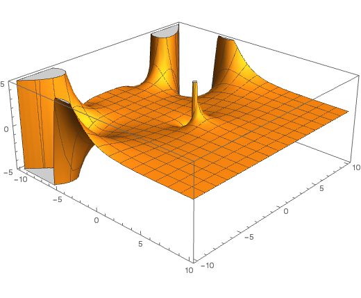
 USD for its resolution, the generalised Riemann hypothesis has far more far-reaching implications. This states that for every Dirichlet L-function, all of its zeroes within the critical strip have real part exactly equal to ½. Since the Riemann zeta function is the simplest example of a Dirichlet L-function, the ordinary Riemann hypothesis is subsumed by the generalised Riemann hypothesis.
 satisfying:
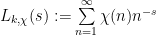
 , with
  and
and  coprime, is necessarily either a prime, a prime power, or twice a prime power.
 . This is, unfortunately, rather slow.
 . If the number is prime, it correctly claims that it is prime. If it is composite, however, it can lie with probability 1/4. In practice, running this test with many randomly-chosen initial parameters will give a result with sufficiently high probability that it is useful in practice (e.g. in cryptography).
 applications of Miller-Rabin are sufficient to guarantee primality, and therefore that there exists a deterministic algorithm with running time
  , noticeably faster than AKS. The