
Last time, we briefly mentioned the high-level differences between Stockfish and Leela Chess.
To recap, Stockfish evaluates about 100 million positions per second using rudimentary heuristics, whereas Leela Chess evaluates 40 000 positions per second using a deep neural network trained from millions of games of self-play. They also use different tree search approaches: Stockfish uses a variant of alpha-beta pruning, whereas Leela Chess uses Monte Carlo tree search.
An important recent change to Stockfish was to introduce a neural network to evaluate the positions in the search tree, instead of just relying on hardcoded heuristics. It’s still much simpler than Leela Chess’s neural network, and only slows down Stockfish to exploring 50 million positions per second.
The real cleverness of Stockfish’s neural network is that it’s an efficiently-updatable neural network (NNUE). Specifically, it’s a simple feedforward network with:
- a large (10.5M parameters!) input layer, illustrated below, that can utilise two different levels of sparsity for computational efficiency;
- three much smaller layers (with 17.5k parameters in total) which are evaluated densely using vector instructions;
- a single scalar output to give a numerical score for the position, indicating how favourable it is for the player about to move.
Everything is done using integer arithmetic, with 16-bit weights in the first layer and 8-bit weights in the remaining layers.
The input layer
Let’s begin by studying the first — and most interesting — layer. Here’s an illustration I made using Wolfram Mathematica:
The inputs to the layer are two sparse binary arrays, each consisting of 41024 elements. It may seem highly redundant to encode a chess position using 82048 binary features, but this is similar to an approach (called ‘feature crosses’) used in recommender systems.
What are the two sparse binary arrays, and why do they have 41024 features? My preferred way of interpreting these two arrays are as the ‘worldviews’ of the white king and the black king. In particular, the differences are:
- Coordinate systems: because black and white pawns move in opposite directions, the two players need to ‘see the board from opposite angles’. This already happens in regular (human) chess because the two players are seated opposite each other at the chessboard, so one player’s ‘top’ is the other player’s ‘bottom’. If you imagine each player numbering the squares from top to bottom, left to right, then any physical square would be called n by one player and 63 − n by the other player.
- Piece types: instead of viewing the pieces as black or white, a player sees it as either ‘mine’ or ‘theirs’. The 10 non-king piece types are thus {my pawn, their pawn, my knight, their knight, my bishop, their bishop, my rook, their rook, my queen, their queen}.
The reason for these ‘player-relative coordinate systems’ is that it means that Stockfish can use the same neural network irrespective of whether it’s playing as white or black. The network uses both your king’s worldview and your enemy king’s worldview for evaluating a position, because they’re both highly relevant (you want to protect your own king and capture your enemy’s king).
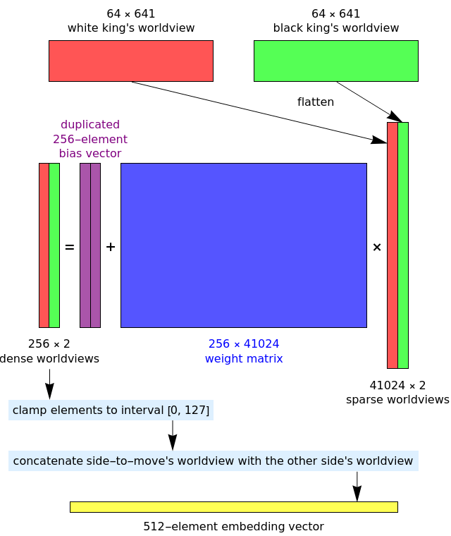
So, why does each worldview have 41024 features? It can be seen as an outer product (or tensor product) of:
- a 64-element feature encoding the position of the king whose worldview this is, in their own coordinate system. This is ‘one-hot encoding’, where exactly one of the 64 entries is ‘1’ and the other 63 entries are ‘0’.
- a 641-element feature encoding, for each of the 64 × 10 ordered pairs (square, piece-type), whether or not that square is occupied by that piece. The 641st element is unused, and is (according to the Chess Programming Wiki) apparently a result of the network being ported from Shogi to chess.
Each of the two 64-by-641 outer product matrices* is then flattened (the matrix is ‘reshaped’ into a vector with the same entries) to yield the corresponding 41024-element ‘sparse worldview’. In the input layer, each of the two 41024-element sparse worldviews are then affinely transformed to form a 256-element ‘dense worldview’.
*Important note: the 41024-element sparse binary arrays are never explicitly materialised, either as a 64-by-641 matrix or as a 41024-element vector. The Stockfish NNUE effectively ‘fuses’ the construction of these sparse vectors with the subsequent affine transformation (described below), updating the 256-element dense worldviews directly when the configuration of pieces on the chessboard is modified.
There are two levels of sparsity which are utilised when computing this affine transformation from 

- the 41024-element implicit vectors are themselves sparse: the number of nonzero elements is equal to the number of non-king pieces on the board.
- moving a piece typically changes very few of the entries of the vector: if it’s a regular non-king move, only 2 entries change; if it’s a non-king move with capture, then 3 entries change.
It’s this second aspect which warrants the name ‘efficiently updatable’: when a move is made (or unmade, since we’re doing a tree search), we only need to add/subtract a few 256-element matrix columns from the resulting ‘dense worldview’ to update it.
Unless a king is moved, this (2 or 3 vector additions/subtractions) beats summing all of the matrix columns corresponding to nonzero entries (up to 30 vector additions), which in turn unconditionally beats doing a regular dense matrix-vector multiplication (41024 vector additions). That is to say, the second-level sparsity is about 10 times more efficient than the first-level sparsity, which is in turn about 1000 times more efficient than naively doing a dense matrix-vector multiplication.
The two dense worldviews are concatenated according to which player is about to move, producing a 512-element vector, which is elementwise clamped to [0, 127]. This elementwise clamping is the nonlinear activation function of the input layer, and (as we’ll describe) the hidden layers use a similar activation function. We can think of this as a ‘clipped ReLU’, which is exactly what the Stockfish source code calls it.
The remaining layers
The two hidden layers each use 8-bit weights and 32-bit biases. The activation function first divides the resulting 32-bit integer by 64 before again clamping to [0, 127], ready to be fed into the next layer. The output layer also uses 8-bit weights and 32-bit biases, but with no nonlinear activation function.
The first hidden layer takes 512 inputs (the clamped concatenated worldviews) and produces 32 outputs. The second hidden layer takes those 32 values as inputs, and again produces 32 outputs. The output layer takes those 32 values as inputs, and produces a single scalar output.
Since these subsequent layers are applied to dense vectors, they can’t use the same ‘efficiently updatable’ approach as the input layer; that’s why they’re necessarily substantially smaller. They can, however, use hardware vectorisation instructions (SSE/AVX) to apply the linear transformation and activation function.
This scalar output is then further postprocessed using other Stockfish heuristics, including taking into account the 50-move rule which isn’t otherwise incorporated into the evaluation function.
Observe that the neural network doesn’t actually have complete information, such as whether a pawn has just moved two squares (relevant to en passant), whether a king is able to castle, and various other information pertaining to the rather complicated rules for determining a draw. This is okay: the network is only being used as a cheap approximate evaluation for a position; when deciding what move to make, Stockfish performs a very deep tree search and only uses this approximate evaluation in the leaves.
Equivalently, you can think of this as being a massive refinement of the approach of ‘look a few moves ahead and see whether either player gains a material or positional advantage’, using a neural network as a much more sophisticated position-aware alternative of crudely ‘counting material’.
This is a neural network, so the weight matrices and bias vectors of the layers were learned by training the network on millions of positions and using backpropagation and a gradient-based optimiser. Of course, for supervised learning, you need a ‘ground truth’ for the network to attempt to learn, which seems somewhat circular: how do you even gather training data? The answer is that you use the classical version of Stockfish to evaluate positions using the deep tree search, and use that as your training data.
In theory, you could then train another copy of the NNUE using the NNUE-enhanced Stockfish as the evaluation function, and then iterate this process. Leela Chess does the same thing: its current network is trained on positions evaluated by using deep lookahead with the previous network as the leaf evaluation function. Note that the construction of the training data is orders of magnitude more expensive than training the network with this data, as you’re doing thousands of evaluations of the previous network (owing to the deep tree search) to construct each item of training data for the new network.
Further reading
The network is described and illustrated on the Chess Programming Wiki, which also has tonnes of references to forum discussions and other references. The first description of an NNUE was a Japanese paper by Yu Nasu (who suggested it for the board game Shogi instead of chess); the paper has since been translated into English and German. There’s also the Stockfish source code, which is very well organised (there’s a directory for the NNUE) and clearly written.
Pingback: The neural network of the stockfish chess engine – Site Title
Interesting! One note is that you wrote “castle” where you probably want to write “rook”.
Amended; thanks. I’ve heard both terms used for the piece, but you’re absolutely right that ‘rook’ is more correct and less ambiguous (since ‘castle’ is already used as a verb).
“Rook” is not “more correct”.
It is correct in absolute terms.
Referring to a Rook as a “Castle” is absolutely incorrect.
ctrl-f for “castle” on https://en.wikipedia.org/wiki/Rook_(chess), it’s clear than in many languages and in casual conversation, a rook can be referred to as a castle.
Castle means something else, obviously.
This is super interesting, thanks! I’d be interested in a post that explains how the affine transformation works, as it’s not clear to me how a 41024 element vector can be transformed into a dense 256 element vector.
It’s multiplication by a 256-by-41024 weight matrix followed by addition of a 256-element bias vector. The weight matrix and bias vector are trained by gradient descent.
Pingback: Assorted topics | Complex Projective 4-Space
But if it’s a non-king move with capture, then 4 entries change, not 3. Why do you say 3? Thanks
Only three entries in the vector change, corresponding to:
1. Removal of moving piece from old location;
2. Addition of moving piece to new location;
3. Removal of captured piece.
This remains true even if the captured piece is removed from a different square than where the moving piece lands (e.g. en passant).
Pingback: Humans Are Hardwired to Cheat. Here’s How We Stop Ourselves. - The New York Folk