I’ve been intending to write about the Leech lattice for a while now. I wanted to ensure that I could actually do it justice, and in particular make it strictly more comprehensive than the Wikipedia and Mathworld articles. The authoritative source on this topic is the book Sphere Packings, Lattices and Groups (Conway and Sloane), which is a compilation of papers by several authors.
A lattice, in this context, is a set of vectors in Euclidean space that form an Abelian group under addition. Equivalently, it is a set of points (including the origin), such that for any two points A and B, there exists a translation mapping A to B and leaving the lattice invariant. For example, the midpoints of the cells of the regular square and hexagonal tilings form lattices in two dimensions, familiar as the Gaussian and Eisenstein integers:
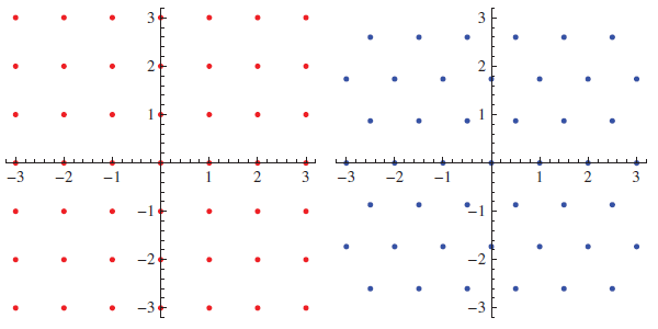
By comparison, this construction applied to the equilateral triangular tiling does not yield a lattice, since there is no translation capable of mapping an up-pointing triangle to a down-pointing one. Nevertheless, the set of points can be expressed as the disjoint union of two hexagonal lattices.
The hexagonal lattice can be regarded as the best lattice in two dimensions, for the following reasons:
- It offers a denser packing of unit discs than any other arrangement;
- It gives a thinner covering of overlapping discs than any other lattice;
- In the packing, each disc touches six others, which is trivially maximal.
The next time a single lattice wins all three awards is in 24 dimensions, with the spectacular Leech lattice. (The E8 lattice in eight dimensions comes close, but is slightly beaten by a lattice called A8* in the covering department.) The rest of this post is primarily concerned with the Leech lattice, although the E8 lattice will undoubtedly be mentioned a few times.
Characterisation and properties
So, what exactly is the Leech lattice? It turns out that it’s the only even integral unimodular lattice with no roots in fewer than 32 dimensions. Each of these terms will take some explaining:
- A lattice, as mentioned at the beginning of this article, is a set of vectors in Euclidean space which is closed under addition.
- A lattice is integral if the dot product of any two vectors is an integer.
- An integral lattice is described as even if the squared norm of any vectors is an even integer. Otherwise, it is an odd integral lattice.
- A lattice is unimodular if the fundamental parallelotope has unit volume, or the determinant of the generating matrix is ±1. Equivalently, the lattice has a density of one point per unit volume. Even integral unimodular lattices only occur in dimensions divisible by 8, with the unique example in 8 dimensions being the E8 lattice.
- For an even unimodular lattice, a root is a vector of squared norm 2. The Leech lattice has none of these, so the shortest nonzero vectors have a squared norm of 4 (or, equivalently, a length of 2).
Because the shortest distance between two lattice points is equal to 2, that means that we can place a ball of unit radius centred on each lattice point. Each sphere touches precisely 196560 others, which is the maximum for 24 dimensions. (The kissing number problem has also been solved in 1, 2, 3, 4 and 8 dimensions, with values of 2, 6, 12, 24 and 240, respectively, attained by the integer lattice, hexagonal lattice, FCC lattice, D4 lattice and E8 lattice, respectively.)
If we enlarge the spheres to a radius of √2, they will overlap and cover all space. Establishing that the covering radius is equal to √2 is non-trivial, and involves analysing all 23 types of deep hole (points maximally distant from lattice points) encountered in the Leech lattice. Each type of deep hole corresponds to one of the 23 other even unimodular 24-dimensional lattices, known as Niemeier lattices.
Coordinate-based constructions
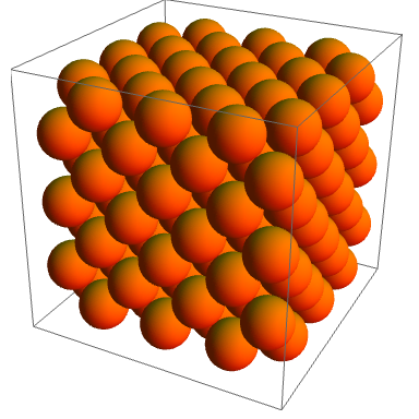
Whilst saying ‘the unique even unimodular lattice in 24 dimensions with no roots’ is sufficient to characterise the Leech lattice, it is appallingly non-constructive. It’s a very complicated lattice, and it’s quite non-trivial to construct the Leech lattice. By comparison, it’s very easy to construct the cubic lattice:
- Points in
 such that all coordinates are integers
and it’s not much harder to construct the D4 lattice:
- Points in
 such that all coordinates are integers and the sum of coordinates is even
or even the E8 lattice:
- Points in
 such that either all coordinates are integers or all coordinates are half-integers, and the sum of all coordinates is even.
Conversely, constructing the Leech lattice using coordinates is really complicated! Even though the following definition is elementary, it involves lots of intermediate steps and is quite complicated indeed:
- Points in
 such that the coordinates are all integers congruent to m modulo 2, the sum of all coordinates is congruent to 4m modulo 8, and such that for each i in {0, 1, …, 11}, the (i + 12)th coordinate is congruent modulo 4 to the sum of the jth coordinates over all j in {0, 1, …, 11} such that (i, j) does not describe an edge of the icosahedron with vertices labelled {0, 1, …, 11}. Then scale the resulting lattice by 1/√8 so that it is unimodular.
This elementary construction was obtained by taking the simplest construction based on the binary Golay code, together with a relatively simple construction of the binary Golay code itself, and combining them. It doesn’t seem to be a particularly motivated construction, though, and there are some simpler ones.
Laminated lattices
This is quite a fun way to create dense lattice sphere packings without much effort. We start with the ordinary integer lattice:
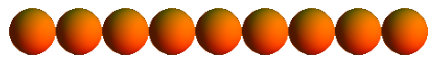
We now add an extra dimension (increasing it from 1 to 2), and place a sphere as low down as possible whilst resting on top of the lattice:
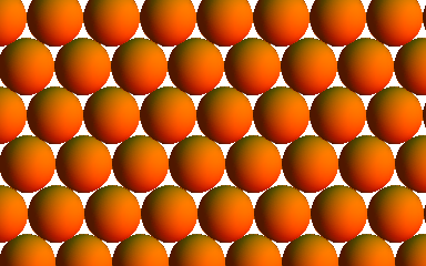
Now take the additive closure (i.e. make it closed under all translations mapping spheres to spheres):
Now imagine it horizontally embedded in three-dimensional space, and add an extra sphere as low down as possible whilst still resting on our hexagonal lattice of spheres. In the image below (plan view), I’ve added six of the spheres of the second layer, and two of the third layer:

Taking the additive closure gives the FCC lattice:
The sequence of laminated lattices obtained in this manner begins Z, A2 (hexagonal), A3 (FCC), D4, D5, E6, E7, E8, and gives rather dense lattices. The laminated lattices in 9 and 10 dimensions are also unique, but there are two types of deep hole in Λ10, giving two different choices for the laminated lattice Λ11. There are three laminated lattices in each of 12 and 13 dimensions, but remarkably instead of getting an exponential explosion of possibilities, all routes converge to a unique laminated lattice in 14 dimensions.
This continues as a nice steady sequence of unique lattices, culminating in Λ24 being the Leech lattice itself! Note that this construction is much simpler than the direct coordinate-based approach using the binary Golay code. However, when one wants to investigate the geometry of the Leech lattice, it is easier to work with the coordinate-based parametrisation.
This is followed by an explosion, as each of the 23 deep holes of the Leech lattice yield different laminated lattices in 25 dimensions, and not much is known about the plethora of laminated lattices in 26 dimensions or above. However, there is a very remarkable periodicity observed in one particular sequence of laminated lattices: the centre density (number of lattice points per unit volume) oscillates with period 24 (and is an even function), where the lattice  is obtained by ‘gluing’
  to the Leech lattice.
Eisenstein integers, Golay codes and Mathieu groups
We have thought of the Leech lattice in its most natural state, which is a 24-dimensional real lattice. Since the complex numbers can be identified with the real plane, this suggests a 12-dimensional complex representation of the Leech lattice. The construction using Gaussian integers is identical to the ordinary 24-dimensional real construction (since the Gaussian integers are isometric to the Cartesian product  ), whereas the Eisenstein construction is distinct.
Instead of using the 24-dimensional binary Golay code over F2, it exploits the 12-dimensional ternary Golay code over F3. The ternary Golay code, whilst named after Golay, was actually discovered a couple of years earlier by a football pool enthusiast (see here). Incidentally, the binary and ternary Golay code constructions of the Leech lattice are two of 23 constructions, one for each Niemeier lattice. Conway and Sloane discuss these ‘holy constructions’ in Sphere Packings, Lattices and Groups.
It’s worth discussing the symmetry groups of these codes. The permutations of the coordinates that fix the binary Golay code form the Mathieu group M24, which has two other sporadic groups (non-Abelian simple groups not of Lie type), M23 and M22, as one- and two-point stabilisers. Similarly, the symmetries of the ternary Golay code give the sporadic group M12, which has M11 as a one-point stabiliser. M21 is isomorphic to PSL(3,4) therefore non-sporadic, and M10 isn’t even simple.
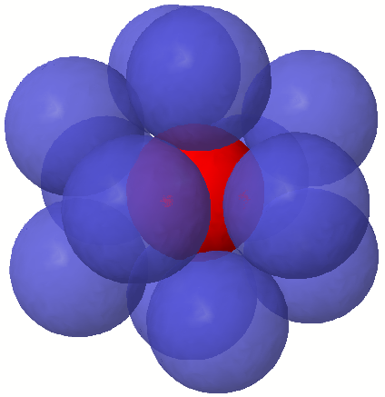
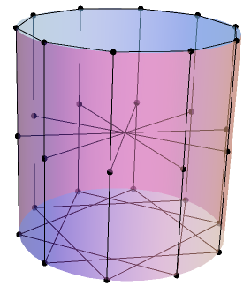
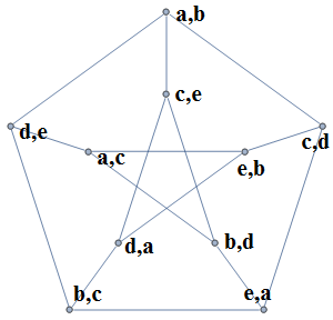
M12 has a nice construction based on the icosahedron. We place twelve ball-bearings around a central sphere (above), corresponding to the vertices of an icosahedron. An inverted twist is an operation where you choose a ball-bearing and its five neighbours, rotate them by 72°, and reflect the arrangement of ball-bearings in the centre of the central sphere. M12 is the group generated by an even number of inverted twists.
M24 can be constructed by a gadget known as the Miracle Octad Generator, which I’ll be explaining in more detail in about a fortnight. For M12, there is a smaller gadget known as the miniMOG (or ‘kitten’, alluding to the fact that ‘mog’ is an informal term for a cat!).
Icosians and the E8 lattice
So far, we have seen that there are real and complex constructions of the Leech lattice. There are also two quaternionic constructions, one of which is boring and analogous to the real and complex constructions. Instead, we’ll describe the more exciting construction, involving the (non-commutative) ring of icosians.
The icosians are a beautiful ring of quaternions with a large degree of symmetry. They are dense in the quaternions, and share some similarities with the integral elements of the quadratic field ![\mathbb{Q}[\sqrt{5}]](https://s0.wp.com/latex.php?latex=%5Cmathbb%7BQ%7D%5B%5Csqrt%7B5%7D%5D&bg=ffffff&fg=000&s=0&c=20201002) in the complex numbers. Whilst this quadratic field can be used to construct the Penrose tilings with fivefold symmetry, the icosians can be used to construct a four-dimensional quasicrystal with the H4 symmetry group possessed by the 120-cell.
in the complex numbers. Whilst this quadratic field can be used to construct the Penrose tilings with fivefold symmetry, the icosians can be used to construct a four-dimensional quasicrystal with the H4 symmetry group possessed by the 120-cell.
The icosians are finite sums of unit icosians, of which there are 120. These include the 24 Hurwitz integers together with the 96 even permutations of ½(0, ±1, ±ψ, ±φ), where φ and ψ are the golden ratio and its Galois conjugate. The unit icosians under multiplication form the binary icosahedral group of order 120, which is the double cover of the icosahedral group.
It is trivial to observe that every icosian is of the form [(a + b√5) + (c + d√5)i + (e + f√5)j + (g + h√5)k], where the variables are rational numbers. This is an icosian if and only if the vector (a, b, c, d, e, f, g, h) lies in a particular scaled and rotated copy of the E8 lattice. We can think of this as a bijection θ from the icosians to the points of the E8 lattice.
Then the Leech lattice can be described as (θ(x), θ(y), θ(z)), where x + y + z = 0 (mod h) and x = y = z (mod h*), where h = ½(−√5 + i + j + k) and h* is its conjugate. We also have a dense three-dimensional quaternionic lattice, L, which is formed by the corresponding points (x, y, z).
Observe that the point symmetry group of the icosians is H4, of order 14400, whereas the point symmetry group of the E8 lattice is the Weyl group of E8, of order 696729600. Hence, there is no reason to assume that L has the same symmetry group as the Leech lattice (described later), and indeed it doesn’t. Whereas the symmetries of the Leech lattice form the double-cover of Conway’s sporadic group Co1, the symmetries of L form the double-cover of the Hall-Janko sporadic group J2. Similarly, the symmetries of the complex Leech lattice yield a setuple cover of the Suzuki sporadic group.
Theta series and automorphism group
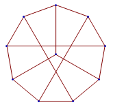
To motivate the discussion of theta series, consider Problem 354 from the Project Euler website. This features a scaling of a hexagonal lattice, where the shortest vectors have squared norm 3 (so the Voronoi hexagons have a side length of 1). They provide a nice picture of this lattice:

The theta series is (the generating function of) the sequence giving the number of points at a specified squared distance. So, in this case, we obtain the theta series  . The Project Euler problem asks how many of these coefficients below some large finite order are equal to 450.
The theta series of the square lattice gives the number of ways to express an integer as the sum of two squares of (not necessarily positive) integers. For the Leech lattice, the number of vectors of squared norm 2m is equal to  , where τ is the Ramanujan tau function and σ11 gives the sum of eleventh powers of divisors.
The first few terms of the theta series of the Leech lattice (A008408) are 1, 0, 196560, 16773120, 398034000, and so on. John Conway observed that the 398034000 vectors of squared norm 8 naturally partition into 8292375 ‘frames’ of 48 vectors positioned at the vertices of an orthoplex (generalised octahedron). Before we divide all vectors by √8 in the coordinate-based construction of the Leech lattice, one of these frames comprises all permutations of (±8,0,0,0,0,0,0,0,0,0,0,0,0,0,0,0,0,0,0,0,0,0,0,0).
The automorphism group is transitive on these coordinate frames, and fixing a coordinate frame gives a subgroup 2^12.M24, corresponding to permutations and sign changes fixing the binary Golay code. By the Orbit-Stabiliser theorem, we recover the size of the automorphism group:
8292375 × 244823040 × 4096 = 8315553613086720000
This group is equal to its own automorphism group. It has a normal subgroup of order 2 (namely its centre, {±I}); the quotient with respect to this is Conway’s sporadic group Co1. The sporadic groups Co2 and Co3 are obtained by fixing additional points. We can also obtain many other sporadic groups in this manner, two of which are described in the next section.
Higman-Sims graph and McLaughlin graph
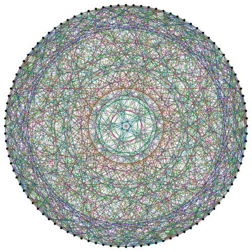
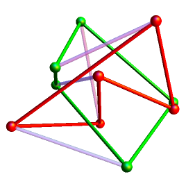
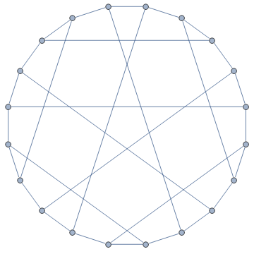
Take three lattice points that form the vertices of a triangle with side lengths of {2, √6, √6}. There are 100 lattice points of minimal distance 2 from all three of these three vertices. Consider these 100 points, and join two points with an edge if the distance is √6. The result is the Higman-Sims graph on 100 vertices. Claudio Rocchini produced the following drawing:
The Higman-Sims graph contains other exceptional graphs embedded within it. There are 352 ways that the vertices can be partitioned into two copies of the Hoffman-Singleton graph. Removing a vertex of the Higman-Sims graph together with its 22 neighbours gives the M22 graph.
We can also obtain the 275-vertex McLaughlin graph, by applying the same construction to a {2, 2, √6} triangle instead of a {2, √6, √6} triangle. The automorphism groups of the Higman-Sims graph and McLaughlin graph are the double covers of two more sporadic groups, the McLaughlin group and the Higman-Sims group.
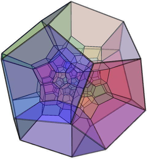
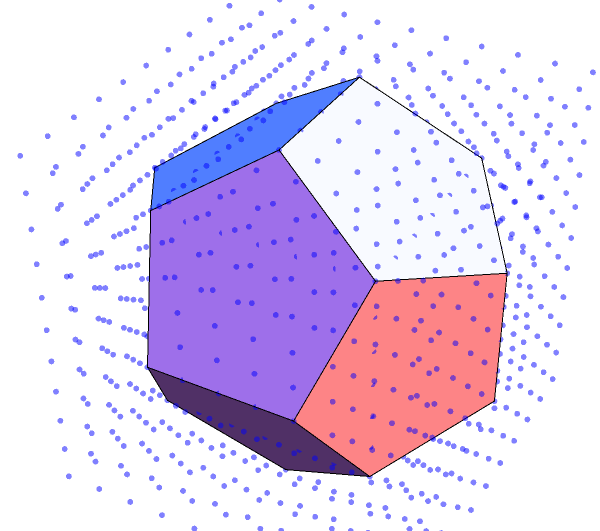
If we take the convex hull of the 240 shortest vectors in the E8 lattice, we obtain the beautiful semiregular Gosset E8 polytope. The convex hull of the 196560 shortest vectors in the Leech lattice is a much more complicated object, but recently its structure was analysed. For each facet of the polytope, the authors construct a graph based on the lengths of its edges. The connected components of these graphs include:
Lorentzian lattices, string theory and the Monster Lie algebra
I was going to include this with the other constructions of the Leech lattice, but I’ve postponed discussion until now due to its depth, abstractness and amount of conjecture.
An elegant construction of the Leech lattice embeds it in (25+1)-dimensional Minkowski spacetime. In this spacetime, we use 25 spatial coordinates and one temporal coordinate, separated by a vertical line. We endow the space with an ‘inner product’ with signature (+, +, …, +|−).
The Lorentzian lattice II(25,1) consists of points such that:
- All coordinates are integers or all half-integers;
- The sum of coordinates is even.
The Leech lattice can be obtained from this by taking the lattice points r such that r.r = 2 and r.w = −1, where w = (0, 1, 2, 3, 4, …, 18, 19, 20, 21, 22, 23, 24, −70) is the Weyl vector, and ‘flattening’ it into Euclidean space whilst preserving the squared distances between points. Remarkably, w is a lightlike vector, since 0² + 1² + … + 24² = 70², as discovered by Edouard Lucas.
The Lorentzian lattice II(9, 1) is also of interest, being intimately related to the 9-dimensional hyperbolic tessellation which completes the sequence {triangular prism, rectified* 4-simplex, demipenteract, E6 polytope, E7 polytope, E8 polytope, E8 lattice, …} of exceptional semiregular polytopes. However, II(9, 1) and II(17, 1) are not as exceptional as II(25, 1), since their Weyl vectors are not lightlike and the corresponding constructions give finite Coxeter-Dynkin diagrams instead of a copy of the Leech lattice.
Conway et al defined an infinite-dimensional Lie algebra based on the Leech roots (those vectors r such that r.r = 2 and r.w = −1), conjecturing that the Monster group occurs naturally as a subquotient of the automorphism group of a sub-algebra. An explicit Monster Lie algebra could be created by applying a particular string-theoretic theorem to a vertex algebra defined by Richard Borcherds.
People such as Stephen Wolfram, Konrad Zuse and Ed Fredkin proposed that our universe is a cellular automaton. One of the major criticisms is that, whilst cellular automata on hexagonal grids can exhibit large-scale SO(2) symmetry (lattice gases are examples), they lack Lorentz invariance. This problem could possibly be circumvented by cellular automata on Lorentzian lattices such as II(9,1) or II(25,1), which exhibit a discrete group of symmetries including Lorentz transformations. Indeed, a particularly well-chosen cellular automaton on II(9,1) or II(25,1) would be a discretised version of 10- or 26-dimensional string theory.
(This article apparently has precisely 3000 words, making it the longest cp4space post so far…)


 . Everything else you have to prove yourself.
 . This asserts that
  , then we can find antipodal points x and y such that f(x) = f(y).
 theorem to easy corollaries. (Of course, these theorems were almost certainly used in establishing the Classification, so this would be logically circular.)

 and subsequent terms are defined by
  , and summarised in the following spiral of equilateral triangles:
 beneath
  . This is because the spiral was designed for the Padovan sequence, which is to the Perrin sequence as the Fibonacci sequence is to the Lucas sequence. This analogy can be made precise by considering the closed form of the Perrin sequence:
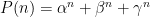
 modulo p.
 , which gives p multiplied by some symmetric polynomial (as all non-trivial multinomial coefficients are divisible by p), which in turn can be expressed as a polynomial in the elementary symmetric polynomials (thanks to Newton’s theorem), which are all integers (by Vieta’s formulae). This result is a massive generalisation of the


 , where V is the desired volume of cream.

 , the continued fraction of which is shown below:
![\sqrt{19} = [4; 2, 1, 3, 1, 2, 8, 2, 1, 3, 1, 2, 8, \dots]](https://s0.wp.com/latex.php?latex=%5Csqrt%7B19%7D+%3D+%5B4%3B+2%2C+1%2C+3%2C+1%2C+2%2C+8%2C+2%2C+1%2C+3%2C+1%2C+2%2C+8%2C+%5Cdots%5D&bg=ffffff&fg=000&s=0&c=20201002) , where the sequence (2, 1, 3, 1, 2, 8) is repeated indefinitely.
, where the sequence (2, 1, 3, 1, 2, 8) is repeated indefinitely.![e = [2; 1, 2, 1, 1, 4, 1, 1, 6, 1, 1, 8, 1, \dots]](https://s0.wp.com/latex.php?latex=e+%3D+%5B2%3B+1%2C+2%2C+1%2C+1%2C+4%2C+1%2C+1%2C+6%2C+1%2C+1%2C+8%2C+1%2C+%5Cdots%5D&bg=ffffff&fg=000&s=0&c=20201002) , whereas others seem to exhibit no obvious patterns, such as π. However, this article is concerned with algebraic numbers rather than transcendental ones, so the next cases to explore are roots of cubics.
, whereas others seem to exhibit no obvious patterns, such as π. However, this article is concerned with algebraic numbers rather than transcendental ones, so the next cases to explore are roots of cubics.
 is significant, as
 ![\mathbb{Q}[\sqrt{-163}]](https://s0.wp.com/latex.php?latex=%5Cmathbb%7BQ%7D%5B%5Csqrt%7B-163%7D%5D&bg=ffffff&fg=000&s=0&c=20201002) is a unique factorisation domain). The reason for the large partial quotients in the continued fraction expansion was explained by Stark, who incidentally was the first person to correctly prove Gauss’s conjecture that the Heegner numbers are precisely {1, 2, 3, 7, 11, 19, 43, 67, 163}.
is a unique factorisation domain). The reason for the large partial quotients in the continued fraction expansion was explained by Stark, who incidentally was the first person to correctly prove Gauss’s conjecture that the Heegner numbers are precisely {1, 2, 3, 7, 11, 19, 43, 67, 163}.