|cp4space| = 100

This is the 100th article on cp4space, and is inspired by a discussion last night with Gabriel Gendler.

Triangle centres with complex numbers

Suppose we have a triangle in the Euclidean plane \mathbb{R}^2. We can identify the Euclidean plane with the complex plane, and represent the triangle by a set of three complex numbers (one for each vertex). I’ll call these complex numbers x, y and z (corresponding to vertices A, B and C, respectively). We’ll now consider a few interesting points in the plane of the triangle:

triangle-centres

The centroid, G, is the easiest triangle centre to express. It’s simply G(x,y,z) = \frac{1}{3}(x+y+z), which is the arithmetic mean of the three vertices. Here, we consider triangle centres to be functions from \mathbb{C}^3 to \mathbb{C}, which takes the three vertices and returns that triangle centre.

The circumcentre, O, is somewhat more difficult to find. It’s the intersection of the three perpendicular bisectors (shown in red in the diagram above), and we can solve simultaneous linear equations to obtain an expression for the circumcentre.

circumcentre

The orthocentre, H, and the nine-point centre, T, are expressible as simple linear combinations of O and G. For instance, H(x,y,z) = 3G(x,y,z) - 2O(x,y,z) and T(x,y,z) = \frac{1}{2}(H(x,y,z) + O(x,y,z)). These points lie on the Euler line, as you can see in the diagram.

Finally, we can also get a simple expression for the symmedian point (either by considering areal coordinates or harmonic quadrilaterals, both of which are explained in MODA).

Algebraically indistinguishable triangle centres

Consider the Steiner inellipse. This is the largest ellipse that can be contained within a triangle, or (equivalently) the image of the incircle of an equilateral triangle after it has been hit with an affine transformation to become the triangle of interest. Probably the easiest way to explain is with a diagram:

Steiner inellipse — diagram courtesy of Claudio Rocchini

The diagram shows the two foci of the ellipse, f_1 and f_2. It is a remarkable fact that the quadratic polynomial with f_1 and f_2 as roots is the derivative of the cubic polynomial with x,y,z as roots. This gives us the following expression:

focus-equation

Of course, we can now solve this quadratic:

focus-formula

This is a multi-valued function, which gives both foci. It is impossible to create an algebraic expression that gives one focus but not the other; they are roots of the same minimal polynomial with coefficients in \mathbb{Z}[x][y][z][x^{\star}][y^{\star}][z^{\star}]. Points with this property (for general fields) are known as Galois conjugates.

The two foci in the previous expression are the same when the radicand (thing being square-rooted) is equal to zero, i.e. when x^2 + y^2 + z^2 = xy + yz + zx. This is equivalent to the triangle being equilateral.

Tritangential circles

The foci of the Steiner inellipse constitute a pair of Galois conjugates. There are other interesting points that belong to larger sets of Galois conjugates. Consider the four circles that are tangent to all three sides of the triangle:

tritangential

The centres of these circles, I, I_A, I_B, I_C, are all roots of the same minimal polynomial, namely this horrible quartic in w:

incentre

Here, I’ve used Σ_alt to indicate the alternating sum over permutations of (x, y, z). This is like the symmetric sum, but where the sign of each term is determined by the permutation of the parity. For example, the circumcentre is given by alt[x y y*]/alt[x y*].

Transcendental triangle centres

The triangle centres (and other points) we’ve explored so far can be given as the roots of polynomials with coefficients in \mathbb{Z}[x][y][z][x^{\star}][y^{\star}][z^{\star}]. Some triangle centres, however, have no such expressions. One particularly interesting example is the Hofstadter point, X_360. Let the Cevian AX_360 intersect the line BC at D; this splits it in the ratio BD : DC = \angle ABC : \angle BCA. You can immediately spot that this is really bizarre, since a ratio between lengths is identified with a ratio between angles.

Posted in Uncategorized | Leave a comment

Sphere packings, lattices and fruits

I’m going to start by describing a game that seems completely unrelated to sphere packing. The Conway-Hamming game involves a half-infinite row of green apples, each of which can either point up or down:

grapples

In any configuration, all but finitely many green apples (occasionally referred to as ‘grapples’) point upwards. The game proceeds as follows:

  • Players alternate taking turns. If a player is incapable of moving, he/she loses.
  • Each turn, a player flips the orientation of between 1 and 3 apples, where the leftmost of those apples must change from pointing down to up.

It’s clear that this process must eventually terminate. Specifically, we can represent each configuration by a non-negative integer, where each 1 in the binary representation corresponds to an apple pointing down. For instance, the configuration above is represented by 51.

The sequence of losing positions is given by the sequence {0, 15, 51, 60, 85, 90, 102, 105, 150, 153, 165, 170, 195, 204, 240, 255, …} (A075928 in the OEIS). Specifically, we construct this sequence term-by-term, where each term in the sequence is the smallest natural number which differs from all of the previous terms by a Hamming distance of at least 4. (Hamming distance is the number of positions in which the binary representations of two integers differ.)

There’s actually a quick method of verifying whether a sequence of apples is a losing position. We write down the binary representations of the positions of each down-pointing apple. For instance, in the first diagram, we have apples in positions 0, 1, 4 and 5.

binary

We then look at each of the columns. (I’ve shown four here, although there are actually infinitely many columns consisting entirely of ‘0’s extending to the left.) The fact that this is a losing position is equivalent to the following statement:

  • In each column, there are an even number of ‘1’s and an even number of ‘0’s.

Error-correcting codes

The losing positions in the Conway-Hamming apple-flipping game correspond to ‘codewords’ in an error-correcting code known as the Hamming code. Suppose Alice sends Bob a codeword, namely a sequence of apples corresponding to a losing position:

grapples

Eve, who is notorious for eating forbidden fruits and attempting to disrupt private communication between Alice and Bob, decides to devour up to three of the apples whilst leaving the others untouched.

eaten-grapples

Amazingly, Bob can actually recover the original codeword from this partial information. If Eve eats four apples, however, some genuine information is lost. Inverting an apple is as bad as eating two apples (in a technical sense which I’ll elaborate upon later), so inverting two apples would also cause problems for Bob.

A variant of the game is where there are 24 apples (instead of infinitely many), and you’re allowed to flip up to seven apples (instead of merely three). The 4096 losing positions correspond to codewords in a very special code known as the binary Golay code. It is generated by the following generator matrix (over the finite field F_2):

000000000000000011111111
000000000000111100001111
000000000011001100110011
000000000101010101010101
000000001001011001101001
000000110000001101010110
000001010000010101100011
000010010000011000111010
000100010001000101111000
001000010001001000011101
010000010001010001001110
100000010001011100100100

Permuting the rows and columns of this matrix results in various equivalent codes. For instance, here is another equally valid matrix:

The left half is the identity matrix; the right half is the complement of the adjacency matrix of the icosahedron. The automorphism group of a binary Golay code (i.e. the permutations of the 24 bits that map codewords to codewords) is the Mathieu group M24. It’s also involved in a particular construction of the Leech lattice, which is in turn used to construct the famous Monster group.

The binary Golay code is even better than the Hamming codes, functioning even if Eve eats up to seven apples. Since it is so efficient, the Golay code was used by the Voyager probes to send photographic information back to Earth. That’s the only practical application of sporadic simple groups of which I know.

Checking and repairing codewords can be done through a pencil-and-paper algorithm known as the Miracle Octad Generator. This, confusingly, has the same acronym as the Mathematical Olympiad for Girls. I intend to write a cp4space post on these subjects later, although I’ll take this opportunity to segue onto the topic of UK mathematical olympiads and wish the best of luck to everyone who sat the BMO2 exam yesterday.

The \mathbb{R}_{\geq 0}^n game

(Yes, I’ve been informed how to embed LaTeX directly into cp4space posts.)

Here’s a game I’ve designed, inspired by Conway’s apple-flipping game. The game position is a n-tuple of non-negative reals (where n is fixed for a particular game). For instance, a possible configuration in the game for n = 3 is (0, 28/5, π). These can be visualised as coordinates in Euclidean space.

On each turn, you’re allowed to move to a position as long as it’s a (Euclidean) distance of less than 1 away from the current position, and that the new position lexicographically precedes the previous one. In other words, (a, b, c) → (d, e, f) is a valid move if and only if both of these conditions hold:

  • (a-d)^2 + (b-e)^2 + (c-f)^2 < 1
  • (a > d), or (a = d, b > e), or (a = d, b = e, c > f).

The losing positions for n = 3 are the centres of the spheres in the hexagonal close packing, which is similar to the arrangements of oranges favoured by greengrocers.

The FCC lattice, which locally resembles the hexagonal close packing

The FCC lattice, which locally resembles the hexagonal close packing

For n = 2, the basic hexagonal lattice gives the losing positions. As for n = 1, it should be obvious that the integer points are precisely the losing positions (if you’re not in a losing position, the winning strategy is to replace x with floor(x) on each of your turns until your opponent is left with 0).

Posted in Uncategorized | Leave a comment

Cipher 14: Remorse

The previous cipher seems to remain unsolved, even though it is indeed solvable. It was originally created by a hermit living in the Adirondack mountains, and was first deciphered by Dave Greene. He subsequently wrote a message in the cipher and passed it to me as a challenge, which I managed to decrypt in a couple of days.

Anyway, here’s this week’s cipher.

2AAA2A22AA22222AAA22A2AA22AA2AA22A2A22AA2AAAAAA222AA2A22A22
22AAAAAA222AA22AA2A22A2AAA222AAA2A22A22AAA2222A2222AA2A22A2
AA22AA2AA22A2A22A2222AA2222AAAA2222A222AAA222AAA22AAA2222A2
AA22AAA22A2AA22A2A2AA2AAA2A222AA22222AAA2AA2A2AAA2A22AA22A2
AA2A222A2AA2AA2A22A2AAA222AA22AA2A22222AA222AA2A22AAA2AAAA2
2AAA2A22AAA2222AAA2AAA222A2AAAA222AA2A2A2AA2222AAA2AA2A222A
2A22AAA22A2A2A22AAAA2AAAA22AAA2AAAA2222A222AAAAAA2222A2AAAA
A222AA2A2AA2AAAA222A2AAAAA2A222A2AAAA22222AA22AA222A2AAAA22
AAA2222AA22AA2222A2222AAAAA222AA2AAA2A222A2A22AA22AAAA2A222
AA222A222A2A222A2AA2AAAA222A2AA22A2AA22AA2A22A22A2A22AA22A2
AA2A2A22A222AAA2222A2222A2222AAAA22AAAAAA2A22222A222AA2A222
AA2A2A2AAA22AAA2AAAA2222AA2A2AA2AAAA222222AAA2AAA22A2A2AA2A
22A2222AA22222AA2A22AA2A222A2AAAAA2AAA22A2AA2AA2A2AA2AAA2AA
2A2A2AA22AA22A2AAAAA22AAA222AAA2AAAA222A222AA2A2A22AAA222A2
22A22A2A2222AAA2A2AAA222A2AA222A22A2AA2AAA2A2AAA2A222AAA2A2
2AA2AAAAA2AAAA2A22A2AAA2A2222AAAAA2AAA2A22A22A2AA2AAA22A2AA
A222A2AA22AA2A2222AA2A22A2222AAA2A2A22A222A2AAA2AA2A22AAA2A
2AA22222A2AA2AA22A2AAAA22A22AA2A2AA222AAAAAA2AA222AAAA2A2AA
22AA22A2AA2A2222A222AA2A222AAAAAA2AAA2222AAA2A22AA2AAAAA2AA

This is just a string, by the way, rather than a matrix. And here’s a completely arbitrary picture of a rod connecting two wheels:

subtle-hint

Good luck, and enjoy!

Posted in Ciphers | Leave a comment

Visualising complex functions

Tim Large suggested to me a new idea of how to render meromorphic functions on the complex plane. Basically, we draw the surface of the Earth on the Riemann sphere (the codomain of the function), and colour each point on the complex plane according to the image of that point under the function.

Excited by this prospect, I set to work programming it. The simplest function is the identity function, which gives the following complex plot (apologies for the blurry polar regions; I used a relatively low-resolution image):

The identity function, f(z) = z

The identity function, f(z) = z

Zeros of functions are rendered as copies of Antarctica. For example, the function f(z) = (z/2)^7 − 1 has seven roots, and thus seven Antarcticas, positioned at the vertices of a regular heptagon of circumradius 2.

The function f(z) = (z/2)^7 - 1, with seven roots at the vertices of a regular heptagon

The function f(z) = (z/2)^7 – 1, with seven roots at the vertices of a regular heptagon

It has seven-fold symmetry about the origin since it is a polynomial function of z^7. Similarly, the function f(z) = z^3 has three-fold symmetry, as we can see below:

The function f(z) = z^3, with three-fold rotational symmetry and a triple root

The function f(z) = z^3, with three-fold rotational symmetry and a triple root

Note that the Antarctica in the centre of this plot has three protrusions, rather than just one, due to it being a triple root. This allows one to very easily observe the multiplicity of a root in such a visualisation of the complex plane. For instance, the polynomial f(z) = (z/2 − 1)^2(z/2 + 1)^3 is shown below:

A complex polynomial with a double-root at 2 and a triple-root at -2.

A complex polynomial with a double root at 2 and a triple root at -2

Functions other than polynomials

So far, all of our functions have been polynomials. Other functions, such as sine and cosine, are more interesting due to the infinity of roots:

The function f(z) = sin(z), demonstrating periodicity parallel to the real axis

The function f(z) = sin(z), demonstrating periodicity parallel to the real axis

There are visible copies of Antarctica at −π, 0 and π. The cosine function is the same, but shifted slightly. The two-fold rotational symmetry means that it is an even function:

The function f(z) = cos(z), showing rotational symmetry

The function f(z) = cos(z), showing rotational symmetry

We can have more bizarre functions, such as the Gamma function, which have many poles (points mapped to infinity).

The Gamma function, a generalisation of the factorial function, with poles at non-positive integers

The Gamma function, a generalisation of the factorial function, with poles at non-positive integers

The Weierstrass elliptic function has a regular lattice of poles, together with two interleaved lattices of zeros. These appear as Arctic tundras and Antarcticas, respectively.

A Weierstrass elliptic function, exhibiting double periodicity

A Weierstrass elliptic function, exhibiting double periodicity

Unfortunately, the poles are rendered poorly due to the texture functionality in Mathematica (it doesn’t realise that the map should be treated as a sphere). I could rectify the situation by using the Image command instead of the RegionPlot, but this would require the use of compiled functions which are not supported on the Wolfram Demonstrations Project.

Non-meromorphic functions

Note that all of the things we’ve seen so far are conformal maps, which preserve angles and orientations. This is a property of all meromorphic complex functions, and means that shapes aren’t locally distorted. If we choose a function which is analytic in the conjugate of z, such as inversion in the circle of radius 2 (f(z) = 4/z*), then the orientations are reversed:

Inversion in the circle |z| = 2

Inversion in the circle |z| = 2

We can tell that this is an anticonformal map, since the British Isles (and everything else!) have been reflected. Worse still are maps which are neither conformal nor anticonformal, since you get weird distortion effects. For example, the absolute value function just has the positive real line as its image, and circles around the origin are mapped to the same value. This creates a ‘target’, where the outermost green band is the intersection of England with the Greenwich Meridian, revolved into an annulus:

Plot of the absolute value function, f(z) = |z|

Plot of the absolute value function, f(z) = |z|

Similarly, Re(z) creates vertical lines, and Im(z) creates horizontal lines.

Posted in Uncategorized | Leave a comment

Ordinal music

The most popular music video of last year is, arguably, Gangnam Style by the famous Korean artist, Ψ. One of the noteworthy features is the presence of ‘accumulation points’ in the music; these occur at 1:07 and 2:29 in the video:

[youtube=http://www.youtube.com/watch?v=9bZkp7q19f0]

Also, the notes in the song are well-ordered, meaning that every set of notes has an earliest element. Indeed, since there are two limit points, the song has order type 2ω + n, where n is the (finite) number of notes after 2:29 in the video.

The night before last, this inspired me to produce music corresponding to a larger infinite ordinal. ω^2 limit points actually sound effective, but when you approach larger limit ordinals such as ω^3 and ω^4, it degenerates into an absolute cacophany. As a proof of concept, I decided to produce the sound of ω^4.

omega4

The scale above represents the entire duration (3:39) of the music, with a linear scale showing certain ordinals marked on it. The first clap you can hear is ‘1’, followed shortly by ‘2’, ‘3’, and all of the other positive integers before reaching a limit point at ω. The entire process is repeated again and again, resulting in limits of limits, such as ω^2 (0:10 in the sound file) and ω^3 (0:46). The music ends at ω^4, although it is possible in principle to produce ordinal music corresponding to any countable ordinal. Most pieces of popular music merely have finite ordinals, with Gangnam Style being a rare exception.

Supertasks

Performing an infinite number of operations in a finite amount of time (such as producing music corresponding to ω) is a transfinite process known as a supertask. For instance, a computer capable of doing an elementary operation in 1/2 of a second, and the next in 1/4 of a second, and the third in 1/8 of a second, can effectively solve the halting problem in 1 second. Such a computer is known as a Zeno machine, since it resembles Zeno’s paradox.

Posted in Uncategorized | Leave a comment

Origami

Firstly, I’ll take this opportunity to wish James Cranch a marvellous 30th birthday.

This post was inspired by the conception of a new ‘origami society’ at Trinity. Having never tried it before, it took me a while to decipher the instructions for the construction of a dragon.

dragon

There are rather restrictive constraints on what possible patterns of folds can be realised. Firstly, arrangements of folds are represented as plane graphs (known as ‘crease patterns’) with two distinct types of edges, namely ‘mountain folds’ and ‘valley folds’. There is actually a third type of edge, a ‘boundary edge’, since we’re dealing with a finite square rather than R^2; the boundary edges form a cycle such that all other vertices lie in the closed subset of the plane bounded by this cycle.

  • Maekawa’s theorem: Each non-boundary vertex must have even degree 2n, such that there are either n + 1 valley folds and n − 1 mountain folds, or vice-versa. As a consequence of the even degree property, the dual graph (or, more pedantically, the induced subgraph of the dual graph obtained by removing the vertex at infinity) has a chromatic number of 2.

This is the only combinatorial restriction, and yields graphs such as this one:

meakawa

There are, however, more geometrical constraints.

  • Kawasaki’s theorem: the sum of the alternate angles around each interior vertex is π. This is a well-defined concept, since Maekawa’s theorem forces the degree of each interior vertex to be even. Also, the configuration must be realisable in Euclidean geometry.

Finally, there is the constraint that the three-dimensional embedding of the folded paper does not self-intersect. This is much more difficult to verify from the diagram than the other two properties.

Postulates

Since origami requires precision, it would be ideal to be able to produce exact crease patterns. This can be accomplished with a pencil, compass and straightedge, as in Euclidean constructions. Basically, the operations achievable with compass and straightedge are:

  1. Given two points, A and B, construct the unique line passing through A and B;
  2. Given two points, A and B, construct the unique circle centred on A and passing through B;
  3. Given two curves which intersect in finitely many points, construct these points of intersection.

It’s not too difficult to show that these operations are equivalent to solving a quadratic given its coefficients. Three famous classical problems, namely ‘doubling the cube’, ‘trisecting the angle’ and ‘squaring the circle’, are unsolvable with these operations (proof: Galois theory for the first two, and transcendentality of pi for the third).

It can be shown via Galois theory that the nth roots of unity can be constructed if and only if n is a product of a power of two and distinct primes of the form 2^k + 1 (i.e. Fermat primes). For instance, Gauss managed to express exp(2πi/17) in terms of square-roots, thus effectively constructing the regular 17-gon.

However, this seems to be digressing somewhat from the original topic of origami. It is overkill to add three new instruments (a pencil, straightedge and compass) to our arsenal, since origami alone can be used for geometrical constructions. Even though circles cannot be constructed for obvious reasons, it is a remarkable fact that we can still construct all of the same points as with the compass and straightedge. Indeed, as will be revealed shortly, a proper superset of those points are origami-constructible.

The ordinary Euclidean constructions are replaced with seven different postulates, known as Huzita-Hatori axioms (despite not actually being axioms).

  1. Given two points, A and B, we can construct a unique fold (line) passing through both of them;
  2. Given two points, A and B, we can construct a unique fold mapping one of them to the other (the perpendicular bisector);
  3. Given two lines, l and l‘, we can construct a fold (two if the lines intersect, or one if they’re parallel) mapping one of them to the other (angle bisector);
  4. Given a line l and a point P not incident with l, we can construct a unique fold passing through P and perpendicular to l;
  5. Given two points A and B and a line l, we can construct a fold passing through A and mapping B onto l;
  6. Given two points, P_1 and P_2, and two lines, l_1 and l_2, we can construct a fold capable of mapping P_1 onto l_1 and P_2 onto l_2;
  7. Given a point A and two lines, l and l‘, we can construct a fold perpendicular to l‘ mapping A onto l.

The sixth postulate is the powerful one, which (in conjunction with the others) enables the general cubic to be solved. This solves both the problems of trisecting the angle and doubling the cube, and allows the construction of nth roots of unity if and only if n is a product of a power of two, a power of three and distinct Pierpont primes.

It is conceivable that someone could write an origami version of Euclid’s Elements. Also, this would be more powerful than Euclid: Morley’s angle trisector theorem cannot be proved by compass and straightedge, since the equilateral triangle cannot be constructed in general, but is within the power of origami.

Posted in Uncategorized | Leave a comment

Cipher 13: Intercardinal

As rasterised images invariably lose quality, this particular cipher is in the form of a PDF document. Click on the link to Cipher XIII to open it.


Posted in Ciphers | Leave a comment

Cayley-Bacharach applications

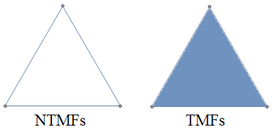
The Cayley-Bacharach theorem in projective geometry states that if two cubics share nine points (in sufficiently general position) and a third cubic passes through eight of those points, then it also passes through the ninth. Here, ‘sufficiently general position’ means that as long as you’re not deliberately stupid with applying this theorem, it will work.

I’ve heard this referred to as a ‘super-theorem’, because its main use is to prove simpler theorems. Firstly, note this very important fact:

  • The union of a degree-m and a degree-n algebraic curve is a degree-(n+m) algebraic curve.

So, for cubics, we can have either an irreducible cubic such as an elliptic curve, or the union of a conic and a line, or indeed the union of three lines. In most applications, we don’t use the full force of Cayley-Bacharach, and concentrate instead on these ‘degenerate’ cases.

Pascal’s theorem (and converse)

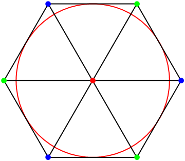
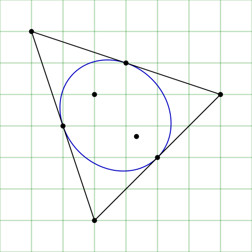
Pascal’s theorem states that if we inscribe a hexagon in a conic, the extensions of opposite sides intersect at three collinear points. The hexagon can self-intersect, such as the following example:

pascal-hexagon

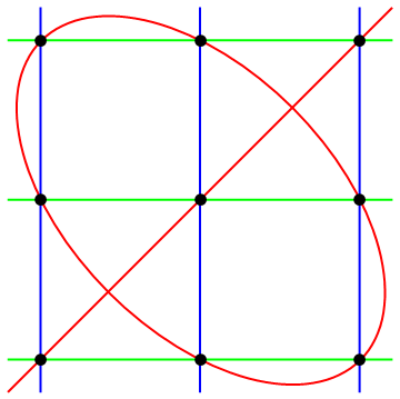
I’ve coloured each cubic in a different colour, such that the nine points are triple intersections. If we lack a single piece of information (such as a concurrency or collinearity) but know that all the other pieces of information hold, we can deduce the final piece of information through Cayley-Bacharach. For instance, the statement of Pascal’s theorem says that the red line exists, and the converse states that the red conic exists.

To determine on which branch of the cubic the point lies (either the conic or the line), we can just apply Bezout’s theorem.

Projective dual: Brianchon’s theorem

Once we have Pascal’s theorem, we can take poles and polars about an arbitrary conic to obtain the projective dual theorem. In projective duality, we interchange lines and points, whereas conics remain conics. Concurrency of lines corresponds to collinearity of points, and so on.

The projective dual of Pascal’s theorem is called Brianchon’s theorem, which states that a hexagon circumscribed about a conic has concurrent diagonals. I’ve colour-coordinated this diagram to correspond with the diagram of Pascal’s theorem; the black lines were originally black points, and the coloured points were originally lines of that colour.

brianchon

We can tell that this is a projective dual of a C-B corollary rather than a C-B corollary itself, because the lines are black and the points are colourful.

Both Pascal’s theorem and Brianchon’s theorem have special ‘degenerate’ cases. If the conic in Pascal’s theorem degenerates into a pair of lines, we obtain Pappus’s theorem instead. This is also a direct corollary of Cayley-Bacharach, for obvious reasons.

In the same way that Pappus is a degenerate case of Pascal, we can view Pascal as a degenerate case of the theorem obtained by replacing the red conic and line with a single elliptic curve. This associativity law is used in elliptic curve cryptography, and more recreationally in my elliptic curve calculator. It is the most difficult part of showing that the points on an elliptic curve form a group under a geometric operation.

Radical-axis theorem and pivot theorem

When we apply Cayley-Bacharach, we actually use the complex projective plane rather than the ordinary Euclidean plane. There are two invisible ‘circular points at infinity’, through which all circles pass. Using these, we can derive some theorems involving circles from Cayley-Bacharach. Only seven of the points are visible here; the other two are the circular points.

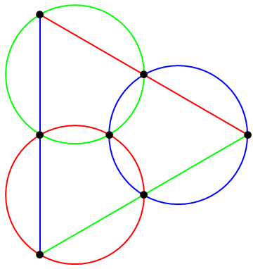
With three circles and three lines, there are two distinct theorems. Firstly, the pivot theorem:

pivot-theorem

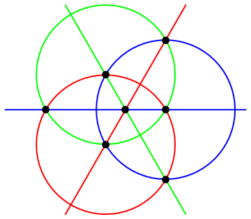
We also obtain the radical-axis theorem in this way:

radical-axis

Circle inversion

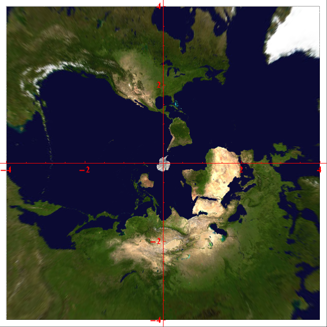
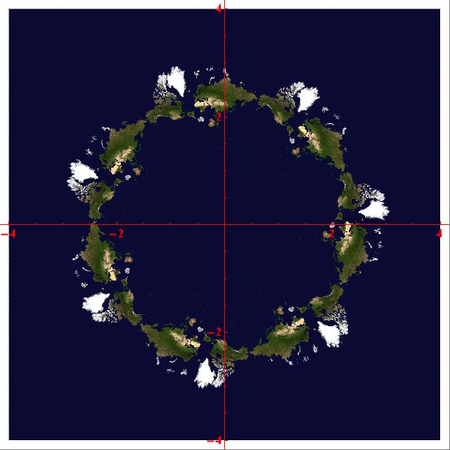
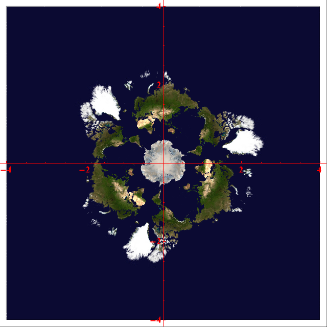
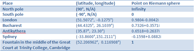
When we’re dealing with circles and lines rather than arbitrary conics, we can concentrate on the real Euclidean plane and extend it to give the Riemann sphere, or complex projective line. This is quite a sneaky trick to switch seamlessly between these two universes, but we can get away with it here. Inverting the pivot theorem yields Miquel’s theorem. This states that if we have eight points and ‘faces’ correspond to concyclic points, then five faces of a cube determine the sixth face:

miquel

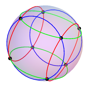
The diagram above was obtained by stereographic projection, so that the cubic nature can easily be appreciated. The radical axis theorem treats the six ‘diagonal’ planes inside a cube instead of the six faces. In the very rare instances where both apply simultaneously, we get the famous orthocentric configuration.

Quartic Cayley-Bacharach

It turns out that there is a generalisation of Miquel’s theorem to eight conics and sixteen points, but this requires the quartic analogue of Cayley-Bacharach to prove. I’ll leave this particular one as an exercise to the reader, and instead use QCB to derive some other beautiful results. There was a particularly elegant problem posted on Art of Problem Solving, the solution to which I’ll describe here.

Firstly, it’s necessary to know the statement of quartic Cayley-Bacharch. If we have 16 sufficiently-general-position points lying on two quartics, and a third quartic passes through 13 of those points, then it also passes through the other 3. In particular, if we need to prove that eight points to lie on a conic, five of them automatically do and we can get the other three through Cayley-Bacharach. Let’s have a look at the AoPS problem:

aops

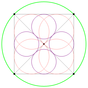
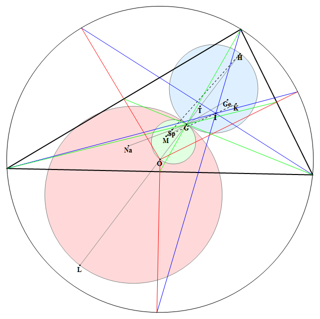
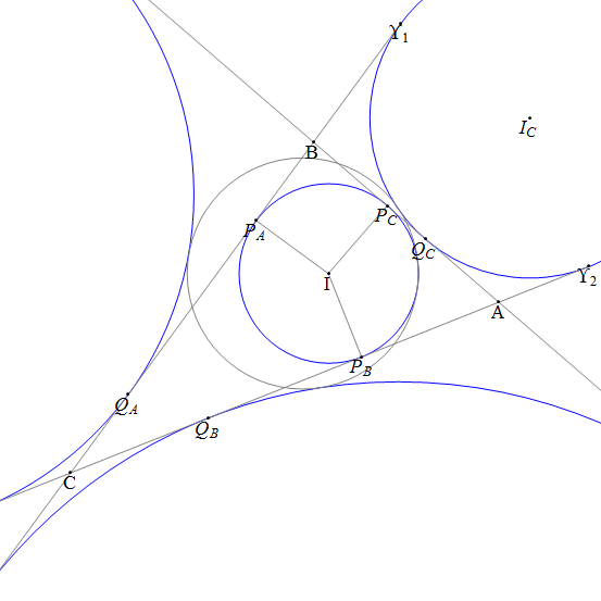
We want to show that the centres of the eight pink/purple circles lie on a conic. We’ll apply the fact that they lie on the angle bisectors of the triangles. Indeed, once we’ve drawn the angle bisectors, we can forget about the grey lines and pink/purple circles completely:

aops2

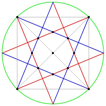
The red and blue angle bisectors intersect to give the eight incentres. However, they also appear to converge on the circumference of the circle to give another four points. This is not a coincidence, and can be deduced from the converse of ‘equal arcs subtend equal angles’. These sixteen points lie on the blue quartic and the red quartic, and we can also draw a green conic through five of the remaining eight points. Quartic Cayley-Bacharach then reveals that the last three points also lie on this conic:

aops3

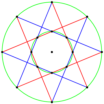
This diagram is a generalisation of Pascal’s theorem, which is a corollary of generalised Cayley-Bacharach. In particular, if we have a 2n-gon inscribed in a conic, and colour alternate edges red and blue, the remaining n^2 − 2n points lie on an algebraic curve of degree n − 2. This is explored in a paper by Gabriel Katz.

Solving an AMS problem

We’ll solve a non-trivial olympiad-style problem using as much pure projective geometry as possible. This differs completely from any ordinary way of solving the problem, although it’s somewhat neater (the standard solution has horrible Menelaus bashes and so forth).

ams-q6

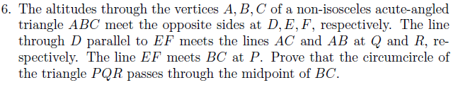
Notice that Q and R are defined in quite a contrived way, so we’ll see if we can learn more about these points. It’s always good to draw a diagram in these contexts; I’ll leave it relatively uncluttered and just include F, E, B, C, Q and R (these are the only ones we’ll require at this stage).

ams1

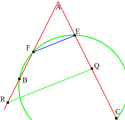
FE and QR meet at a point on the line at infinity, which is thus collinear with the two circular points. Colour the line at infinity red. We already have that the green circle exists (and has diameter BC, by Thales’ theorem), so we can conclude that BCRQ lie on a blue circle by Cayley-Bacharach. You could alternatively use an angle chase, but that’s too boring for cp4space.

The orthocentre exists; hence, (P,D;B,C) is a harmonic range. Consequently, the circle on diameter PM is the inverse of the line AD (polar of P) with respect to the circle on diameter BC (centre M). So, AD is the radical axis of circles on diameters PM and BC. This means we can just apply a degenerate case of the radical axis theorem to the points {D, Q, R, B, C, P, M} to deduce that {M, P, Q, R} are indeed concyclic.
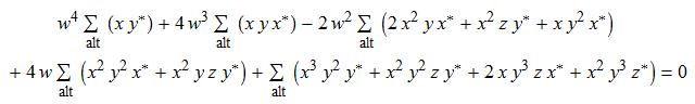
Posted in Uncategorized | 7 Comments

Non-trivial mutual friends

Suppose we have a set of n people, and we want to encapsulate a particular relation which holds between them. For instance, the people who have featured on the cipher solvers page can be represented by a directed acyclic graph. We have a directed edge A → B if person A dominates person B, that is to say that A solved a proper superset of the ciphers solved by B. There is also the transitivity property: A → B and B → C together imply A → C. I have removed these extraneous edges from the digraph to improve clarity.

digraph-2013-01-18

Sam Cappleman-Lynes and Joseph Myers are known as maximal elements, as no-one dominates either of them. The entire graph is an example of a partially ordered set, or poset.

For more symmetrical relationships, it is better to use an undirected graph. For instance, we can connect two people (vertices) with an edge if they are friends with each other. There is no convenient way to analyse the entire global friendship graph, although social networks provide good approximations. There has been a paper examining this graph and revealing certain interesting properties; for instance, the largest connected component of a particular network features about 700 million people, whereas the second largest contains roughly 2000 people.

From graphs to hypergraphs

Vishal Patil and I realised that an ordinary graph is insufficient to embody certain concepts in social communities. For instance, if A, B and C are mutual friends, they would be represented by the cycle graph C_3. However, we can make a more subtle distinction: do the three people know each other merely pairwise, or have they all met simultaneously? By using something called a hypergraph, we can distinguish between non-trivial and trivial mutual friends:

mutual-friends

Trivial mutual friends are far more common, and are just three people who know each other having been together simultaneously. Non-trivial mutual friends (NTMFs, a term originally coined by Vishal, which has later passed into widespread use) are much rarer; the canonical example provided by Vishal was that someone he met at school later encountered James Aaronson on a tour of Israel. An analogy is that 6, 10 and 15 are pairwise non-coprime, but are coprime when considered together.

The set of hypergraphs which can arise is far smaller than the powerset of the powerset of the number of people. In particular, certain constraints must be obeyed:

  • If A is an element of the hypergraph, and B is a subset of A, then B is also an element of the hypergraph (obviously);
  • For every vertex v, the singleton set {v} belongs to the hypergraph (people vacuously know themselves).

Hypergraphs obeying this restriction are known as abstract simplicial complexes. The number of abstract simplicial complexes on n labelled vertices is given by {1, 2, 9, 114, …} (sequence A006126 in the OEIS). Equipped with this new idea of considering abstract simplicial complexes, Vishal and I considered more complicated structures that could arise.

If A, B and C are non-trivial mutual friends (i.e. {A, B}, {B, C} and {C, A} belong to the hypergraph, but {A, B, C} does not), then we can describe them as being either unique non-trivial mutual friends (UNTMFs) or non-unique non-trivial mutual friends (NUNTMFs). A set of three NTMFs are described as unique if there is no person D such that {A, D}, {B, D} and {C, D} belong to the hypergraph. Our first example was a set of three UNMTFs, as no-one else knows Vishal, James and their mutual friend.

Non-unique non-trivial mutual friends

An example of non-unique non-trivial mutual friends includes me, Vishal, Jovan and Katya. The simplical complex corresponding to our acquaintancy is given below:

non-unique

As with all NUNTMFs, the situation is represented by a hollow tetrahedron with between zero and four faces (a solid tetrahedron would correspond to a set of four trivial mutual friends). The possibilities are shown below:

NUNTMFs

Below each of these simplicial complexes is a number called the encounter count. This is the minimum number of encounters necessary for this relationship to be satisfied, i.e. the number of maximal elements in the partially ordered set of simplices under inclusion. Trivial mutual friends have an encounter count of 1.

Counter-unique configurations

The extremal cases of either zero or four triplets of TMFs in a set of four NUNTMFs are very symmetrical, so Vishal decided upon a new name. Rather than describing the configurations as the tongue-twisting ‘encountercountextremal non-unique’, he decided upon the much more manageable ‘counter-unique’. I don’t know of any real-life examples of counter-unique NTMFs, although I have been in a partial tetrahedron where five of the edges and none of the faces were established:

almost-counter-unique

The way in which this peculiar object formed was quite surprising. Radley and I knew each other ab initio, as did Suzy and Miranda. Slightly later, but still ages ago, Suzy met me (thus creating a path graph on four vertices). Radley subsequently met Miranda at their college (Homerton), thus completing a 4-cycle. The fifth edge was completed when Radley met Suzy at the Cambridge Union Society, and we were tantalisingly close to becoming counter-unique non-trivial mutual friends. However, when three of us went to a formal (evening dinner) at Trinity, a face was created and thus the opportunity destroyed.

If you’ve been affected by any of the issues in this blog post, please mention so in the ‘comments’ section below. I would particularly like to hear if you know any real-life examples of counter-unique non-trivial mutual friends, and ideally how they became established.

Posted in Uncategorized | 24 Comments

Assorted stuff

This post contains miscellaneous topics which don’t deserve individual articles, but are still worth mentioning nonetheless.

Stereographic map projections

When you look at a map of the world, the most common projection is the Mercator projection. This is a conformal map, which means that angles between curves are preserved and there is no local distortion. Another possible map projection, which conformally mapping the sphere to the (extended complex) plane, is stereographic projection. One possible formula is given below:

trinitycentric

The expression above converts latitude and longitude (in degrees) to a complex number, corresponding to a point on the (extended) complex plane. This is a stereographic projection, thus angles are preserved and circles drawn on the surface of the Earth map to circles on the complex plane. Moreover, meridians are mapped to rays through the origin. Here are a few places on Earth, together with their latitude/longitude and complex representation:

locations

The numbers given in bold are exact values; others are approximations only. The point corresponding to -1 on the complex plane is just off of the north-east coast of Semisopochnoi Island, Alaska. The real line is the great circle passing through the north pole, south pole and Trinity.

Ambigram equations

An ambigram is a centrally symmetric motif, typically displaying a word. For instance, one example from ambigram.com is the word ‘ambigram’ itself, rendered below:

I was wondering whether it would be possible to write a true statement in first-order logic together with logical conjunctions and arithmetic operations, which also functions as an ambigram. There are trivial examples such as 0 = 0. I subsequently found a slightly less trivial ambigram, namely this one:

ambigram-equation

Of course, it would be more exciting to have a statement involving logical connectives and quantifiers. Because the universal and existential quantifiers rotate to give the letters ‘A’ and ‘E’, respectively, ambigrams in first-order logic are really quite contrived. I managed to cheat slightly by using the carat ^ to denote exponentiation, and for its rotation to be the symbol for logical disjunction.

ambigram

This reads as ‘0 equals 0, or there exists S, such that there exists A, such that for all E, we have that S times E to the power of 0 equals 0’. This is true, as the thing to the left of the ‘or’ is true and the thing to the right is grammatically correct. From here, you can easily derive more complicated examples by replacing the first ‘0 = 0’ with any true equation formed from the symbols {(, ), 0, 1, 6, 8, 9, +, ×, −, =}.

Vastly improved Basilisk

In an earlier post, I alluded to the existence of a very large and rather slow (c/69) spaceship in the HighLife cellular automaton. Due to a combined effort involving Dean Hickerson, Matthias Merzenich and me, we have managed to reduce its size considerably and actually build more complicated constructs involving it. These examples can be downloaded and simulated rather quickly in Golly.

If you recall, the previous idea relied on a complicated (8, 8) push reaction and a very simple (4,4) pull reaction, which can be joined together by a massive train of replicator units emulating addition modulo 2. The size of the resulting Basilisk was impractically large, so we endeavoured to optimise it. The first breakthrough came when Matthias Merzenich discovered a far simpler reaction capable of pushing debris by the vector (6, 6). Even when two are composed to yield a (12, 12) push (commensurate with the (4, 4) pull at the opposite end), the period is still marginally smaller than the minimum attainable with old technology.

matthias-push

The arrangement with symmetry group isomorphic to V4 is repeatedly pushed northwest by the train of replicators. Due to the small period, the length of the minimal Basilisk found by my search program ended up around 15000 replicator units. Basilisks can be combined together to yield rakes capable of periodically emitting gliders. I have uploaded an example comprising six cooperating Basilisks.

Even more ambitious was the concept of a static arrangement that periodically emits Basilisks at regular intervals. The most familiar analogue is the standard Gosperian glider gun in Life:

Of course, Basilisks are massive compared with the tiny gliders emitted by Bill Gosper’s gun, and too complicated and chaotic to assemble incrementally. Eventually, I thought of an alternative idea, which is to bombard the Basilisk with a few gliders to catalyse replication — by the linearity of addition modulo 2, any replicator track will copy itself when left to its own devices. Then, another wave of gliders is required to sterilise the replicators to yield ordinary Basilisks. By using high-period glider guns (thanks go to Dean Hickerson for providing them) to do this automatically, we have a machine for breeding Basilisks (download Golly file).

basilisk-gun

The mechanism (repeated breeding and sterilisation) is completely different from any other spaceship gun in any cellular automaton, and only works for XOR-extendable spaceships.

Posted in Uncategorized | Leave a comment