Complex Projective 4-Space

This is the sequel to the previous article defining ultrafilters and establishing basic properties thereof. Again, the proof of Hindman’s theorem is from Imre Leader’s lecture course on Ramsey theory.

It seems initially paradoxical that ultrafilters are actually useful. After all, it is impossible to explicitly describe a non-principal ultrafilter, as the proof of their existence relies on the axiom of choice. Nevertheless, they have found many applications throughout mathematics, especially in topology and Ramsey theory.

There is a hierarchy of filters with increasingly strong properties:

• Ordinary filters (useful in topology to generalise the notion of a sequence to apply to spaces which are not first-countable; originally, nets were used instead, but they have been largely obsoleted by filters)
• Ultrafilters
• Non-principal ultrafilters
• Idempotent ultrafilters
• Minimal idempotent ultrafilters

Principal ultrafilters are not particularly interesting or useful, so we shall begin by seeing what we can achieve when armed with a non-principal ultrafilter. Deeper in the article, we shall explore the applications of idempotent and minimal idempotent ultrafilters.

Elections

When there are only two competitors in a democracy (and the electorate has an odd finite cardinality), it is rather trivial to determine the victor. Specifically, the following procedure should be applied:

1. Each person in the electorate ranks the political parties.
2. The votes are aggregated, and the party with the most votes wins.

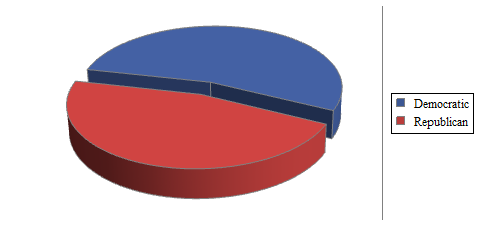
For instance, in the 2008 US election, Barack Obama won with 69498516 votes, whereas the runner-up John McCain had 59948323 votes. Here’s a gratuitous infographic:

This simple majority voting system possesses many desirable qualities (stated in a way to generalise to n political parties):

• Non-dictatorship: No single person has total control over the election.
• Universality: The votes made by the electorate should deterministically determine a total ordering of political parties, the outcome.
• Independence of irrelevant alternatives: If S is a subset of the set of political parties, then the total ordering restricted to S in the outcome should depend only on the total ordering restricted to S in the preferences of each voter.
• Monotonicity: If some subset of the electorate increase the position of a party in their preferences, then this does not decrease the position of that party in the outcome.
• Non-imposition: Any of the n! outcomes (total orderings on the political parties) can be achieved.

Someone called Arrow famously proved that it is impossible to create a similarly ideal voting system when there are three or more political parties. For instance, it is very easy for two parties to have the same number of votes, so the naive majority idea does not generalise.

Hence, in the United Kingdom where there are more than two political parties, it is impossible for any of these sophisticated alternative vote systems to possess all of the desired qualities. Does this mean that we have no hope whatsoever?

Actually, no: there is a subtle caveat, namely that Arrow’s impossibility theorem only holds when the electorate is finite. Otherwise, it breaks down spectacularly. Specifically, we have the following voting system:

1. Let U be a non-principal ultrafilter on the electorate (set of voters).
2. Each voter selects his or her preferred outcome (out of n! possibilities).
3. Precisely one of the n! possible outcomes is favoured by a measure-1 subset of the electorate, with respect to U. This is the overall outcome.

(If a principal ultrafilter were used instead, we would precisely have a dictatorship.)

In conclusion, we have a beautiful voting system where there are no dictators, and no ‘extremist groups’ of finite cardinality can control the outcome, either. Unfortunately it’s non-constructive by virtue of depending on the axiom of choice, but never mind. Non-principal ultrafilters save the day!

Ramsey’s theorem

It’s possible to prove the infinite variant of Ramsey’s theorem (that any k-colouring of the edges of a countably infinite complete graph contains a monochromatic countably infinite complete induced subgraph) using elementary methods. However, there is a proof using ultrafilters which seems slightly cleaner.

In particular, we choose a non-principal ultrafilter U and choose the colour c satisfying (∀U x ∀U y : (x, y) is coloured with c), and intend to find a monochromatic infinite clique of that colour. We construct this sequentially, choosing a vertex x_n with the property that (∀U y : (x_n, y) is coloured with c) and such that the edges joining x_n to each of the previously-selected vertices {x_1, x_2, …, x_(n−1)} are all the correct colour. Repeat ad infinitum.

Now that we have an algorithm, we now need to prove that it actually works. How do we know that we can always choose such an x_n? Well, x_n must satisfy precisely the following conditions:

• ∀U y : (x_n, y) is coloured with c;
• (x_1, x_n) is coloured with c;
• …
• (x_(n−1), x_n) is coloured with c.

For each of these conditions considered in isolation, a measure-1 set of vertices have the desired property. There are finitely many such conditions, so their intersection also has measure 1, and in particular is non-empty. Hence, the inductive step of the proof is complete.

This proof also generalises in an obvious way to prove Ramsey’s theorem for hypergraphs (where the ‘edges’ are r-subsets instead of 2-subsets, for some fixed r). By comparison, proving the hypergraph Ramsey theorem using elementary methods involves a clever induction on the value of r.

The finite version of Ramsey’s theorem can then be deduced from the infinite version using a compactness argument. Unlike the finitary inductive proof of Ramsey’s theorem, however, this does not provide an explicit bound on how large a complete graph must be to contain a monochromatic subset of size n.

Hindman’s theorem

We’ve seen a basic application of ultrafilters in Ramsey theory, but it is only slightly easier than the finitary proof and doesn’t really justify developing the theory of ultrafilters. By comparison, the next result (Hindman’s theorem) is very deep, and the most elegant proof relies on the existence of idempotent ultrafilters.

Hindman’s theorem is a massively strengthened version of Schur’s theorem, one of the first results in Ramsey theory:

Schur’s theorem: If we finitely colour the positive integers, we can find x and y such that x, y and x+y are all the same colour.

This is really straightforward to prove. Specifically, we colour the edge (a, b) of the graph on the positive integers according to the colour of |a − b|. Then, by Ramsey’s theorem, we can necessarily find a, b and c such that (a, b), (b, c) and (c, a) are all the same colour (a monochromatic triangle). The result follows immediately.

A strict generalisation is Folkman’s theorem, which states that this is possible with arbitrarily many positive integers:

Folkman’s theorem: If we finitely colour the positive integers, we can find (for any n) integers {x_1, x_2, …, x_n} such that the 2^n − 1 finite sums are all the same colour.

This is not too surprising. The next generalisation is.

Hindman’s theorem: If we finitely colour the positive integers, we can find integers {x_1, x_2, x_3, …} such that all finite sums are the same colour.

So, how do we prove this? It actually follows rather quickly from the existence of an idempotent ultrafilter, U, which we established during the previous article. When we finitely colour the positive integers, precisely one of the colour classes, c, has measure 1 with respect to our idempotent ultrafilter U.

Suppose we have a set S_n = {x_1, x_2, …, x_n} with the property that ∀U y : (all finite sums of {x_1, x_2, …, x_n, y} are coloured with c). Consequently, for all 2^n − 1 finite sums z of distinct elements of S_n, we have the property ∀U y : (z + y is coloured with c). By idempotence, this gives ∀U x : ∀U y : (z + x + y is coloured with c). Taking the intersection of these 2^n − 1 new statements (one for each z) together with the 2^n − 1 old statements ∀U x : (z + x is coloured with c), we obtain the following:

• ∀U x : ∀U y : (all finite sums of {x_1, x_2, …, x_n, x, y} are coloured with c).

So, simply let x_(n+1) be such an x (guaranteed to exist since measure-1 sets are non-empty) and we obtain a proper superset S_(n+1) with the property. Hence, by induction we are done.

Addition and multiplication

Hindman’s theorem has a multiplicative corollary, that we can find an infinite monochromatic set such that all finite products are the same colour (proof: consider powers of two and apply regular Hindman’s theorem). Indeed, a colour class which is measure-1 with respect to a multiplicatively idempotent ultrafilter would have this desired property. The existence of ultrafilters which lie in the topological closures of the sets of additively and multiplicatively idempotent ultrafilters means that we can actually satisfy the additive and multiplicative versions with the same colour class:

• Double Hindman’s theorem: We can find sets S = {x_1, x_2, …} and T = {y_1, y_2, …} such that all finite sums of elements of S and finite products of elements of T are the same colour.

Similarly, there is a double van der Waerden’s theorem. The proof using ultrafilters is the easiest proof, although this can also be achieved using Szemeredi’s theorem (the density analogue of van der Waerden). The proofs of both double Hindman and double van der Waerden (which, if I remember correctly, can be made to apply simultaneously to the same colour class in some grand generalisation!) make use of minimal idempotent ultrafilters. These are idempotent ultrafilters belonging to a minimal ideal in the semigroup (βN, +), and their existence requires another application of Zorn’s lemma beyond what was necessary to prove the existence of bog-standard idempotent ultrafilters.

Other applications of idempotent ultrafilters are given in this MathOverflow discussion.

Ultrafiltered milk

The concept of ultrafiltered milk is rather amusing, to me at least, since (non-principal) ultrafilters are inherently non-constructive and therefore very unlikely to be useful in agriculture. Indeed, it is an unfortunate fact that ultrafiltered milk does, in fact, have absolutely no connection with ultrafilters whatsoever, and it is a mere etymological coincidence.

I assert that the world would be a much better place if ultrafiltered milk actually involved ultrafilters in the production process…

This is the first of a projected two-part series of articles about ultrafilters. The former introduces ultrafilters and establishes various properties about them, so that the latter article can concentrate entirely on applications of ultrafilters.

Much of this material is from Professor Imre Leader’s lecture course on Ramsey theory, notes of which can be obtained from Paul Russell’s website.

I’ve been intending to write about ultrafilters for some time, but, whilst simple to define and manipulate, they are rather abstract objects. I suppose I’ll first give a formal definition, and then attempt to provide a more intuitive interpretation of what an ultrafilter is.

So, an ultrafilter U on a set S is a collection of subsets of S with the following properties:

• If A is in U, then every superset of A is also in U (U is an upset);
• If A and B are in U, then the intersection A ∩ B is also in U;
• Precisely one of A and S\A belongs to U.

The correct way to view ultrafilters is a way to assign a finitely-additive measure to S, where every set has either measure 0 (almost nothing) or measure 1 (almost everything). Then, U is the collection of big (measure-1) subsets of S. The axioms then have entirely intuitive interpretations:

• If A is a big set (has measure 1), then so is every superset of A;
• The union of two measure-0 sets also has measure 0;
• If A has measure 1, its complement has measure 0, and vice-versa.

Very often, we take S to be the set of positive integers, . From the ultrafilter axioms, we can deduce the following:

• If we partition a measure-1 set into finitely many sets, then precisely one of those has measure 1.

There is a notion of a stronger version of an ultrafilter (on necessarily uncountable sets) where ‘finitely’ is replaced with ‘countably’ (thus is a genuine measure in the usual sense), but their existence is equivalent to that of a certain large cardinal called a measurable cardinal for obvious reasons. Anyway, in the remainder of the article we will only consider ultrafilters on the set N of positive integers.

Examples of ultrafilters

When trying to explain ultrafilters, I am compelled to provide a few examples. The easiest examples to provide are the principal (boring) ultrafilters, such as the following:

A set has measure 1 if and only if it contains the number 7.

There is a principal ultrafilter for each natural number n, by replacing 7 with n. Principal ultrafilters are somewhat silly, since they only care about a single element of S. Note that if a finite set has measure 1 with respect to some ultrafilter, then one of its elements must have measure 1 and the ultrafilter must be principal. So, in a non-principal ultrafilter, all measure-1 sets are infinite (as they should be).

Anyway, what’s an example of a non-principal ultrafilter?

It transpires that non-principal (or free) ultrafilters cannot be explicitly constructed, relying heavily on the axiom of choice. We create an ultrafilter U by extending a filter F, which is a strictly weaker notion than that of an ultrafilter. A filter F need only satisfy the following properties:

• The empty set does not belong to F;
• The entire set S does belong to F;
• If A and B belong to F, then so does the intersection;
• If A belongs to F, then so does every superset of A.

Unlike ultrafilters, there are lots of interesting examples of filters. For instance, we can take the filter of cofinite sets, where a set belongs to F if and only if its complement is finite.

There is an obvious partial order on the set of filters, namely inclusion. If a filter is not an ultrafilter, then we can extend it by throwing in another set. If we have a chain (totally-ordered set of filters), then the union is a filter which is an upper bound. Hence, by Zorn’s lemma, we can extend any filter to a maximal filter (an ultrafilter).

Ultrafilters as quantifiers

You are probably aware of the universal quantifier ∀ and the existential quantifier ∃. Given your favourite ultrafilter U, we can define the quantifier ∀U (pronounced ‘for U-most’) as follows:

• ‘∀U x : P(x)’ means ‘P(x) is satisfied by a measure-1 set of x in S’

It has the beautiful property that it distributes over all Boolean operators:

• ∀U x : (P(x) or Q(x)) ⇔ (∀U x : P(x)) or (∀U x : Q(x))
• ∀U x : (P(x) and Q(x)) ⇔ (∀U x : P(x)) and (∀U x : Q(x))
• ∀U x : (not P(x)) ⇔ not (∀U x : P(x))

The first two of these also apply to ∃ and ∀, respectively, but the third applies to neither (∀ and ∃ are interchanged, rather than preserved, when conjugated by logical negation).

Warning: it does not commute with itself (∀U x ∀U y is not the same as ∀U y ∀U x). This again contrasts with the more familiar logical quantifiers.

The Stone-Cech compactification of N

The space of ultrafilters on the positive integers is denoted βN and admits a natural topology. Specifically, we define a base of open sets:

• For every set A of positive integers, let C(A) = {U in βN | A in U} be an open set.

C(N) and C(Ø) are βN and Ø, respectively. The intersection of two base sets, C(A) and C(B), is easily verified to be C(A ∩ B), so this is indeed a base of open sets. A set is open if and only if it is some arbitrary union of base sets. Note that again we have C distributing over everything:

• C(A ∩ B) = C(A) ∩ C(B)
• C(A ∪ B) = C(A) ∪ C(B)
• C(N \ A) = C(N) \ C(A) = βN \ C(A)

In particular, the base sets C(A) are both open and closed.

So, why are we interested in the topology on βN? It transpires that it has several very nice properties:

• Hausdorffness: For two distinct ultrafilters, U and V, we can find a set A such that A belongs to U but not to V. Then, C(A) contains U and C(N\A) contains V. Since C(A) and C(N\A) are disjoint open sets, this means that βN is a Hausdorff space.
• Compactness: Suppose we have a collection P of closed sets, such that the intersection of any finite subset of P is non-empty. It suffices to consider the case where the elements of P are all base sets. Indeed, let P = {C(A) : A in Q}, where Q is a collection of subsets of N, such that any intersection of finitely many elements of Q is non-empty. Let F be the filter of all supersets of elements of Q, and extend it to an ultrafilter U. U must necessarily belong to all elements of P, and therefore their intersection. This establishes the finite intersection property, which is trivially equivalent to topological compactness.
• N is dense in βN: We can embed N in βN by associating the number n with the principal ultrafilter {A in N : n in A}. Then N is a dense subset of βN, since for every non-empty C(A) in the base of open sets, we can choose an arbitrary a in A and observe that the principal ultrafilter on a belongs to C(A). βN is actually the largest compact Hausdorff space in which N is dense, and is called the Stone-Cech compactification of N. It is a surprising fact — which is not too difficult but still non-trivial to prove — that after removing N from βN, we are left with an inseparable space (one with no countable dense subset).

Even though it is very nice from a topological point of view, little is known about βN. Assuming the continuum hypothesis, Parovicenko proved that several topological assumptions are sufficient to characterise βN; conversely, in the absence of the continuum hypothesis, there exist non-homeomorphic spaces satisfying the same properties. Also, if we assume certain large cardinal axioms, then βN has completely different properties than under the (incompatible) assumption of the continuum hypothesis.

Ultrafilter addition and idempotent ultrafilters

Recall that N admits a commutative addition operation. This can be extended to a non-commutative addition on βN, where we define the sum of two ultrafilters as follows:

• U + V = {A ⊆ N | ∀U x ∀V y : x + y in A}

Note that this can easily be verified to satisfy the defining properties of an ultrafilter. This is associative, since (U + V) + W = U + (V + W) = {A ⊆ N | ∀U x ∀V y ∀W z : x + y + z in A}. We can also prove that it is left-continuous, that is to say that U + V is a continuous function of U. Of course, working in a general topological space, there is only one definition of continuity that we’re allowed to use: the pre-image of an open set is open.

It suffices to prove that, for an arbitrary fixed ultrafilter V, the pre-image of C(A) is always open, for every A ⊆ N. So, let’s unpack the definitions:

Note that U + V = {A ⊆ N | ∀U x : (∀V y : x + y in A)}, so the pre-image of C(B) is the set:

• {U in βN | {A ⊆ N | ∀U x : (∀V y : x + y in A)} in C(B)}
• = {U in βN | B in {A ⊆ N | ∀U x : (∀V y : x + y in A)}}
• = {U in βN | ∀U x : (∀V y : x + y in B)}
• = {U in βN | {x in N | (∀V y : x + y in B)} in U}
• = C({x in N | (∀V y : x + y in B)})

which is open, by definition. To summarise, the operation + is associative and left-continuous, and βN is a compact Hausdorff space. We’re now going to forget absolutely everything else about ultrafilters, and prove the following lemma:

The idempotent lemma: If X is a non-empty compact Hausdorff space and + is a left-continuous associative operation, then there exists x in X such that x + x = x.

The proof requires extensive use of Zorn’s lemma.

We firstly consider the collection S of non-empty closed sets Y with the property that Y + Y is a subset of Y. The entire space X is trivially one such example, so our collection S is non-empty. Endow S with the partial order of inclusion.

If we have a chain of such sets, then the intersection is non-empty (since all finite intersections are non-empty, and we are working in a compact Hausdorff space where compact sets are closed and vice-versa) and closed (by virtue of being an intersection of closed sets). So, every chain has a ‘lower bound’ in S and thus we can find a minimal Y by Zorn’s lemma.

Choose an arbitrary x in Y, which we can do by the fact that Y is non-empty. Y + x is the continuous image of a non-empty compact set, thus non-empty and compact. Also, (Y + x) + (Y + x) = Y + Y + x + x, by associativity, which is clearly a subset of Y + x. Hence, Y + x is also in S and is a subset of Y, so Y + x = Y (as otherwise Y + x would be more minimal than Y).

Now define Z = {y in Y | y + x = x}, which is non-empty since Y + x = Y, and Y contains x. It is the pre-image of a singleton set (which must be compact and thus closed) under a continuous function, so is itself closed. If y and y‘ both belong to Z, then (y + y‘) + x = y + (y‘ + x) = y + x = x, so Z + Z is a subset of Z and therefore belongs to S. So Z = Y by minimality of Y.

Hence, since x is in Y, x is in Z and therefore x + x = x, concluding our claim.

Consequently, there must exist an ultrafilter U with U + U = U. It is clear that such an ultrafilter must necessarily be non-principal. U is known as an idempotent ultrafilter. Non-principal ultrafilters themselves already have many applications (as we shall see in the follow-up post), but idempotent ultrafilters are even more useful, powerful and generally awesome. I can imagine that you’re all bursting with excitement in anticipation of the follow-up article, so I shall endeavour to write it as soon as feasibly possible.

(This article is about the axioms concerned with the existence of enormous sets. If you were instead looking for corpulent subordinates of the Pope, then I suggest watching this Monty Python sketch.)

How big is the universe? Ultrafinitists such as Doron Zeilberger reject the Axiom of Infinity, and only allow finite sets. The universe of all finite sets, Vω, is a perfectly consistent set theory, which obeys all of the other axioms of ZFC. It’s not a particularly powerful set theory, though, as we can’t encapsulate the notion of the set of natural numbers.

So, Vω is too small to be consistent with ZFC. It turns out that the smallest universe consistent with ZFC is L, Gödel’s constructible universe, where at each successor stage we take only the sets expressible by first-order formulae ranging over sets in the previous stage. In L, the generalised continuum hypothesis is true, so every cardinality can be obtained by taking unions and powersets. There are other nice corollaries of V = L (the axiom that the entire von Neumann universe is the same as Gödel’s constructible universe) such as the existence of a Suslin tree.

Large cardinals are those with special properties, typically whose existence is not implied by ZFC. Many of these have very complicated set-theoretic definitions, but there are some easier notions related to Ramsey theory. For example, for your favourite ordinal α, the Erdős cardinal κ(α) is the smallest cardinal such that for all n, every 2-colouring of the n-subsets of κ(α) contains a monochromatic set of order type α. If α = ω, for example, then the infinite Ramsey theorem asserts that κ(ω) = .

0# and beyond

Note that if β < α, then the existence of κ(α) implies the existence of κ(β). There’s a property of intermediate strength between the existence of κ(ω1) and the existence of κ(β) for all countable β, namely the rather interesting axiom 0#. 0# is defined as a set of true statements (in L augmented with the symbols {, , …} (one for each natural number) interpreted as cardinalities in V), but it can also be encoded as a set of naturals (by Gödel numbering) or indeed as a real number.

The only problem is that sometimes statements do not necessarily have a prescribed truth value, so 0# is not necessarily well-defined. If 0# exists, then V is much larger than L; otherwise, V can only be very slightly larger than L. So, 0# is really the first large cardinal property that goes beyond V = L.

Beyond 0#, there is a hierarchy of increasingly strong large cardinal properties. At the end of this list are Reinhardt cardinals and strong partition cardinals, which are so strong that they break ZFC (although strong partition cardinals, at least, are consistent with ZF). The strongest large cardinal that is not known to be inconsistent with ZFC is a rank-into-rank cardinal, which is marginally weaker than a Reinhardt cardinal.

Specifically, it asserts the existence of an ordinal γ such that the γth iteration of the von Neumann universe, Vγ, can be non-trivially mapped into itself such that the truth of all first-order statements are preserved. (Such a map must obviously be an injection, as the statement ‘a is not equal to b’ must be preserved for all distinct elements a and b.)

Laver tables

The existence of a rank-into-rank was used by Richard Laver to prove a certain very combinatorial statement. A Laver table of order n is the table of a binary operation satisfying the properties and .

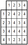
The periodicity of the first row of the Laver table, i.e. the period of  as a function of i, must necessarily be a power of 2. In the example above (n = 2), the first row is (2, 4, 2, 4), which has a period of 2. The period is also an increasing function of n, but it increases extremely slowly. It (sequence A098820) begins as follows:

1, 1, 2, 4, 4, 8, 8, 8, 8, 16, 16, 16, 16, 16, 16, 16, 16, 16, 16, ...

where the number of sixteens is more than A(9), where A(n) is the fast-growing Ackermann function. In general, the point at which the sequence first exceeds 2^m, if it exists, is not a primitive-recursive function of m (eventually dominating the Ackermann function).

The proof that the sequence increases without bound actually relies on the existence of a rank-into-rank cardinal. So, if these things don’t actually exist (which is entirely plausible), then it may be that the sequence is eventually constant. It seems extremely unusual (impossible, surely?) that such a basic combinatorial statement would be independent of ZFC, so it is generally believed that A098820 does indeed grow without bound. But then again, it has not been proved that the existence of a rank-into-rank is consistent with ZFC, and people initially believed otherwise — that the inconsistency proof of Rienhardt cardinals could be adapted to disprove the existence of a rank-into-rank — but all attempts failed miserably so the general concensus is that they are consistent with ZFC.

Is it possible to dissect a square into finitely many pieces, which can then be rearranged to form a disc of equal area?

Note that, unlike in three dimensions where the Banach-Tarski paradox exists, dissections must respect the two-dimensional Banach measure and therefore preserve areas. Hence, it is impossible to rearrange the pieces to form a disc of larger or smaller area than the original square.

Obviously, if the pieces are sufficiently well-behaved (e.g. have simple piecewise-smooth boundaries), then there is no solution; the proof is extremely elementary. In 1989, Laczkovich found an axiom-of-choice-based dissection into approximately 10^50 pieces, answering Tarski’s question in the affirmative.

Anyway, my friend and colleague Tim Hutton, inspired by discussion with his 6-year-old daughter, decided to ask how close you can manage with n non-pathological pieces, for varying values of n. More precisely, he asked the following question:

What is the supremum area a(n) of n interiors of topological discs with piecewise smooth boundary, such that they can be packed in both a circle of unit area and a square of unit area?

It is trivial to observe that as n tends to infinity, a(n) monotonically approaches 1. Also trivial is establishing the value of a(1):

He’s also launched a collaborative project to find dissections giving lower bounds for a(n). For instance, with six pieces it is possible to achieve 0.9860:

Undoubtedly, more can be found on Tim Hutton’s Google+ page.

Consider the following problem:

• Let  be a finite set of positive integers. Suppose we colour the positive integers with k distinct colours. Prove that there exist constants a and b such that is monochromatic.

Initially, this seems as though it should be a pretty difficult problem. After all, the equations are not linear due to the scary exponent b, so we can’t (for example) appeal to Rado’s theorem. However, closer inspection will reveal that at no point are we using the additive structure of the ring of integers, but instead just the multiplicative structure.

And the multiplicative structure of the positive integers is a very simple and ubiquitous object, thanks to the Fundamental Theorem of Arithmetic. In fact, it is rather surprising that its most succinct name is the free commutative monoid on countably many generators. To see this isomorphism, consider the prime factorisation of the integer:

• .

This is a bijection between the positive integers and sequences of non-negative integers of finite support. In particular, it satisfies the delightful prosthaphaeretic property, θ(n m) = θ(n) + θ(m). If we consider the positive rationals instead of the positive integers, then this gives a group isomorphism; without the existence of inverses, however, this is just an isomorphism between monoids.

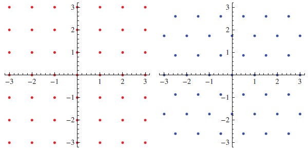
So, what happens when we pass our problem through this monoid isomorphism? We recover the statement of the Gallai-Witt theorem (multi-dimensional generalisation of van der Waerden’s theorem). Specifically, it states that if we have a finite subset S of , then we can find a monochromatic homothetic copy of S in any k-colouring of the lattice.

It is quite amusing to see how many problems on competitions such as the IMO are actually concerned with the free commutative monoid on countably many generators, and have just been pathetically disguised as number-theoretic problems concerned with divisibility. I think that Gallai-Witt is one of the few theorems that obfuscate into a reasonably concise and natural statement rather than a contrived mess under the inverse of θ.

Knot theory

One of the main principles in knot theory is that (directed) knots under the operation of connect sum form a monoid. Here is an example of this operation:

It’s not too difficult to see that when the knots are directed, this is indeed a well-defined operation. Proving that it forms a free commutative monoid is slightly more difficult, involving the following:

• Establishing that anti-knots do not exist;
• Showing that we can uniquely express a knot as a connect sum of irreducibles, up to reordering.

The first part is generally accomplished by the famous Eilenberg-Mazur swindle. As for the second, the proof proceeds by showing that ‘overlapping irreducible knots’ can be further reduced, thus establishing a proof by contradiction. As a result of this, it suffices to only tabulate irreducible (or ‘prime’) knots, as all other knots can be uniquely expressed as a connect sum of prime knots.

Taking the ‘prime’ analogy completely literally, we can (via the free commutative monoid on countably many generators) define an isomorphism φ from the naturals to the set of knots*, such that φ(a b) is the connect sum of φ(a) and φ(b). The exact choice of φ is pretty arbitrary; each φ is uniquely determined by a bijection between the set of primes and the set of prime knots.

* Strictly speaking, the set of tame knots (those with finite complexity). The set of wild knots is uncountable.

Anyway, applying φ to the problem at the beginning of this article gives a third (and much more ridiculous!) equivalent statement of Gallai-Witt:

• Assign to each distinct knot one of k colours. Suppose we have r knots, . Prove that there exists a knot A and a positive integer b such that, when we define the knot M_i to be the connect sum of A with b copies of N_i, the knots form a monochromatic set.

Before we begin, there are a few late items of news worth discussing:

• There is a free edition of Wolfram Mathematica for the Raspberry Pi, an increasingly popular versatile low-cost computer. More details are available over at The Aperiodical.
• The first round of the British Mathematical Olympiad has taken place. Marking is scheduled for the forthcoming weekend, and high scores will be published soon after. Until then, you can see the questions on Joseph Myers’ website.
• The TMS Call My Bluff (mentioned during the previous cp4space post) was won by the freshers’ team. They were winning 4-2, and James Munro gave each team a set of tangled Borromean rings as a tie-breaker (quite literally!). The non-freshers won the tie-breaker, increasing their score to 4-3. Many thanks to all who participated; it was a pleasure to host the event (and not merely because I was entitled to an excess of mince pies and port!).
• You may have noticed the recent Diwali-themed cp4space banner (thanks, by the way, to the CUHCS committee for organising an awesome celebration!). This will soon be replaced with a Saturnalia banner, then a Christmas one, and ultimately the New Year banner. Since cp4space is over a year old, these are very re-usable.

Anyway, you’re probably eagerly anticipating another cp4space article, so here goes:

Sphere eversion

Suppose we have a circle in the plane, and wish to transform it into its reflection by a homotopy (continuous deformation). Moreover, at every point in time, the curve must be an immersion of the circle: it is allowed to smoothly self-intersect, but cannot have any cusps or singularities. Can the transformation be done?

The answer is no: we can approximate such a differentiable map by a smooth one. Then, the total curvature must be preserved during the homotopy, whereas a clockwise circle and anticlockwise circle have opposite total curvatures.

However, for a sphere in three-dimensional space, this proof fails and, remarkably, it is actually possible to evert a sphere. There’s a video explaining the problem and briefly demonstrating the solution discovered by Bill Thurston, who proved that it is possible to perturb an arbitrary homotopy to remove any singularities.

[youtube=http://www.youtube.com/watch?v=R_w4HYXuo9M]

Another solution is symmetric with respect to time, with the half-way model being the Morin surface. If we conjugate a rotation of the Morin surface by 90° with a homotopy transforming a sphere into a Morin surface, then we get the complete sphere eversion. This is more ad hoc than Thurston’s corrugations, and does not generalise easily to more complicated surfaces.

The aforementioned Morin, who is a retired topologist, was blind from the age of six; despite this, he was able to not only find an explicit solution to sphere eversion, but also discover the first parametrisation of Boy’s surface, an immersion of the real projective plane.

Since the real projective plane can be described as a sphere where antipodal points are identified, we can deduce that Boy’s surface has an Euler characteristic of 1. It is also non-orientable, a property it shares with the better-known Klein bottle (which has Euler characteristic 0). Interestingly, the name of the Klein bottle and its common realisation as a bottle with its neck re-entering through a hole and connecting to the base are the result of a German mistranslation.

A very impressive theorem states that any connected compact surface can be identified uniquely up to homeomorphism by the Euler characteristic, orientability and number of boundary components. Hence, they can be described as connected sums of projective planes (‘crosscaps’), tori (‘handles’) and closed discs (‘holes’).

Many theorems in analysis have combinatorial analogues, which turn out to be equivalent (in the sense that one can be derived from the other, and vice-versa, using significantly less maths than is necessary to prove either from first principles). A particularly useful theorem is Brouwer’s fixed-point theorem, which can be proved from its combinatorial discretisation, Sperner’s lemma.

Sperner’s lemma, not to be confused with the similarly-named theorem generalised by Hunter as mentioned in my earlier article about punting in clearings of arbitrarily small Lebesgue measure, is concerned with colouring vertices in a simplicial subdivision of a simplex. In two dimensions, we take an equilateral triangle and cut it into smaller triangles, like so:

We colour each of the vertices with one of three colours (or n + 1 for the n-dimensional version), such that all of the vertices of the original triangle (or simplex) are different colours. Also, if a vertex occurs on the boundary of the simplex, then it must be coloured with the same colour as one of the vertices of the facet in which it resides. (So, for example, any vertices on the bottom edge of the triangle above must be either blue or yellow.)

Then, Sperner’s lemma states that the number of triangles (or simplices) in the subdivision whose vertices are distinct colours (highlighted in grey in the diagram above) is odd. Crucially, that means that there must be at least one such simplex.

In one dimension, the lemma is completely trivial to prove. It states that if we have a finite sequence of vertices coloured red or blue, such that the leftmost vertex is red and the rightmost vertex is blue, then there are an odd number of pairs of adjacent differently-coloured vertices. For instance, the following diagram has five such edges, highlighted in yellow:

Proving Sperner’s lemma involves inducting on the number of dimensions. For instance, the two-dimensional statement can be deduced from the (trivial) one-dimensional statement. We consider the triangulation to be drawn on the surface of a sphere (so the large triangle also constitutes a triangle), and form a subgraph of the dual polyhedron by replacing each triangle with a vertex and connect vertices corresponding to triangles sharing an edge whose endpoints are (red, blue). Now, by Sperner’s lemma in one dimension, the big triangle has odd degree. Hence, by the handshaking lemma, we can find another triangle with odd degree, which must correspond to a triangle where all vertices are differently coloured.

As well as its use in proving Brouwer’s fixed point theorem (mentioned below), Sperner’s lemma is involved in the proof of Monsky’s theorem, that we cannot dissect the unit square into an odd number of triangles of equal area. The proof is reasonably short, but amazingly ingenious. I very much recommend reading it.

Analytical analogue

We aim to prove Brouwer’s fixed point theorem, which states that any continuous function from the closed n-ball to itself must necessarily have a fixed point. An equivalent problem is to show that there is no continuous function f from the closed n-ball to its boundary S such that f restricted to S is the identity function (such an f is called a continuous retraction).

We shall demonstrate this for simplicial subdivisions of regular simplices, which are homeomorphic to balls, and intend to show that any continuous function f sending vertices to vertices (a simplicial map) that is the identity when restricted to the boundary must send one of the simplices in the subdivision to the big simplex.

In particular, let the vertices of the big simplex be {v_0, v_1, v_2, …, v_n}. Then we give a generic vertex w the colour i if f(w) is closer to v_i than any other v_j. After taking a deep breath, we realise that any continuous retraction must violate Sperner’s lemma, thus establishing that continuous retractions do not exist for simplicial subdivisions of regular simplices. And since any continuous function can be approximated by considering its effect on a sequence of progressively more refined simplicial complexes, we are done.

The special case of Brouwer’s fixed point theorem applied to homeomorphisms in three dimensions has a nice physical interpretation. Suppose we have a volume of pumpkin velouté in a glass vase, and stir it crazily in a continuous way. Then the fixed point theorem states that somewhere, a molecule of the velouté is in the same place whence it began.

Midsummer House

Speaking of pumpkin velouté, that was, when punctuated with a la grecque mushrooms and Parmesan gnocchi, the first of eleven courses in a most delightful meal I enjoyed at Midsummer House on Thursday evening. Ordinarily, cp4space does not usually give reviews of double-Michelin-starred restaurants in articles about combinatorial proofs of analytical theorems, but this time I shall make an exception.

Not only was the food incomparably excellent, but also the atmosphere was absolutely perfect. We were seated on two extraordinarily comfortable chairs in the spacious solarium of a quaint Victorian villa overlooking the Cam. The ambient illumination was provided by contemporary candelabra situated around the boundary of the room, providing a warming glow on this late November evening.

Before the amazing dinner began, we were given champagne, canapés* and condiments, the latter of which had, in the case of the other person with whom I was dining, an unusually overwhelming affinity for the table cloth. Fortunately, its act of rebellion was expertly rectified by the means of a supplementary table cloth provided after the course of pumpkin velouté, when its disobedience became known to the brilliantly professional staff.

* Miniature cheese scones and suchlike. I would have added this in parentheses, but decided that a footnote allowed me to do so without interrupting the alliteration.

The second course encompassed mackerel tartare, chervil, fennel and passion fruit, arranged in an aesthetically pleasing symmetrical configuration. This was accompanied by the first of a flight of wines designed to perfectly complement the exquisite dishes.

This was followed by great confusion when a large metal trolley arrived; we were assured that the explanation as to its imposing presence would become apparent in the immediate future. Due to unbridled inquisitiveness, I was compelled to consult the menu to deduce its purpose in life, correctly inferring that it harboured the ‘open coals’ on which the beetroot was to be cooked.

Unsurprisingly, the beetroot was extremely flavoursome, and by far the best beetroot I had ever had the fortune to sample. Indeed, this statement would remain true if ‘beetroot’ were to be replaced by many of the other culinary delights on the menu. Including the course of sautéed scallop, celeriac and truffle. The celeriac was arranged in alternating layers of parallel lines, forming a precise Cartesian grid when viewed from above.

According to the menu, the next course comprised roast quail, shallot purée, grapes, celery and sour dough, positioned on various strata of an interesting bowl, the structure of which was analogous to the discrete energy levels occupied by an electron in a hydrogen atom. This was accompanied by a pleasant surprise, namely the delicacy of quail’s eggs. Unlike most eggs, which are conventionally and eponymously ovoid*, these were spherical. The interior was a luscious yolk.

* The most common explanation for the deviation from a sphere or prolate spheroid is so that, when rolled, the egg travels in a closed path rather than escaping arbitrarily far from the origin and falling from the bird’s nest; this presents an evolutionary advantage.

For the following course, we had a choice between bass and monkfish, and decided upon the latter on the basis that I was already accustomed to the taste of bass. When asked what monkfish was, and due to the temporary cognitive modification that results from having consumed considerably more wine than my opponent, I bluffed with total conviction that they are marine animals, which live totally detached lives in monasteries (and in the immortal words of Meat Loaf, two out of three ain’t bad). She was not fooled by this ruse.

I distinctly remember quince appearing on the menu, as I was asked to describe it and quite satisfyingly was able to respond with ‘a fruit with botanical name Cydonia oblonga‘. (The reason for knowing the Linnaean name of a quince is another story, involving a friend of mine called Quincy, and is far too tangential to describe here.)

The next course was a pousse café, a delicious combination of several liquids of distinct densities, which formed strata in a hemispherical receptacle atop a glass vessel. The uppermost layer, which was delightfully creamy, was peppered with fragmented mint leaves. This was followed by a range of artisanal cheeses.

The penultimate course was an indescribably delectable dessert of lemon posset, lemon espuma and blueberries. In fact, it was so amazingly orgasmically excellent that it would be assigned some non-recursive transfinite ordinal on Vishal Patil’s famous dessert quality scale, which hitherto only ranged from 0 to 10.

The eleventh and final course included caramel, chocolate and chestnuts (ooh, another triple alliteration!), providing an ideal culmination for this fabulous gastronomic experience. It was accompanied by a sweet dessert wine, the seventh of the glasses in the flight of wines, which complemented the course perfectly.

At the end of the meal, which was over three hours of absolute Elysium, we spent a rather long time exploring the balcony, overlooking the river (which would have been moonlit had I had the foresight to ensure that the evening coincided with the correct lunar phase), and enjoying the satisfyingly secluded gardens of this Victorian villa, until ultimately retreating into the Fellows’ Garden of Trinity College…

So, yes, I thoroughly recommend this splendid restaurant. The Empress of TMAS described it as:

‘The nicest forfeit I’ve ever been on’

(Specifically, she agreed to do absolutely anything in return for being removed from the freshers’ team for the Trinity Mathematical Society Call My Bluff — which you should definitely attend on Monday 2nd December — and I decided that this would be appropriately awesome.)

Borsuk-Ulam and Tucker’s lemma

Returning from that rather brief aside, there are other examples of theorems in analysis with combinatorial counterparts. In particular, the Borsuk-Ulam theorem (mentioned in Desert Island Theorems) has Tucker’s lemma as its discrete version.

Yesterday, I attended the UKMT mentoring conference in Murray Edwards College (affectionately abbreviated to ‘Medwards’), which mainly consisted of an excellent dinner in the Fellows’ dining room and informal discussion about various topics. Speaking of mentoring, I recently prepared for one of my mentees a crash course in the application of Gaussian integers to solving certain olympiad-style Diophantine equations.

What follows is an almost verbatim regurgitation of that e-mail.

Brief introduction

So, basically a Gaussian integer is a complex number of the form a + bi, where a and b are both integers. When plotted in the complex plane, they form a square lattice, as shown in the left-hand diagram below.

The hexagonal lattice of blue points is the ring of Eisenstein integers, which shares many of the same interesting properties as the Gaussian integers. Now, the most important fact about Gaussian integers is this:

Gaussian integers are a Unique Factorisation Domain.

The ordinary integers are also a Unique Factorisation Domain, as I’ll explain below.

Unique factorisation domains

Basically, the elements of  (the ring of integers) can be categorised as follows:

• Zero: 0
• Units: +1 and -1
• Irreducibles: +2, -2, +3, -3, +5, -5, +7, -7, +11, -11, …
• Composite numbers: +4, -4, +6, -6, +8, -8, +9, -9, …

Units are defined as elements whose reciprocals also belong to the ring. In particular, every non-zero element in a field is a unit. Irreducibles are defined to be elements that cannot be expressed as a product of two non-units; everything else is composite.

Now, we define a prime to be a number p such that if p|ab, then p|a or p|b. It’s straightforward to show logically that every prime must be an irreducible. It’s very non-trivial to show that the converse holds (that all irreducibles are primes), and there are rings in which this is not the case, such as . But for the integers, this is true, because they form a Principal Ideal Domain.

The integers are also a Unique Factorisation Domain (this follows from the property that all irreducibles are primes), which essentially means that the Fundamental Theorem of Arithmetic holds. Specifically:

Every integer can be uniquely expressed as a product of irreducibles, up to reordering and multiplication by units.

A proof of this from the prime property is given in the bottom-right corner of the second page of this GRM revision sheet I prepared earlier. Anyway, now that I’ve described these concepts in terms of the ordinary integers, I’ll now explain the Gaussian integers.

The Gaussian integers

The Gaussian integers, written Z[sqrt(-1)], also form a PID (hence a UFD), so we have the nice property that all irreducibles are primes. Firstly, we need to identify which elements are units; in this case, they are +1, -1, +i and -i.

Note that the number 2 is not a prime in the Gaussian integers, since (1 + i)(1 – i) = 2, and neither 1 + i nor 1 – i is a unit. 1 + i and 1 – i are irreducibles (and called `associates’ since they differ only by multiplication by a unit, analogous to the irreducibles +3 and -3 in the ordinary integers). In fact, we can show the following:

A positive integer is a Gaussian prime if and only if it is prime (as an ordinary integer) of the form p = 4k + 3.

One direction is easy to prove; p cannot be divisible by any integers >= 2 (by primality), so we need to show that it can’t be expressed as the product of two (complex conjugate) Gaussians, p = (a + bi)(a – bi) = a^2 + b^2. But p is congruent to 3 mod 4, so is not the sum of two squares.

In the other direction, a prime of the form p = 4k + 1 can be expressed of the form a^2 + b^2 = (a + bi)(a – bi), so factorises over the Gaussians and is therefore not a Gaussian primes. There’s a nice proof of this based on Wilson’s theorem, and relying on the notion of Gaussian integers.

It might be informative for you to see what the Gaussian primes look like. Here’s a lovely picture by David Eppstein:

The Gaussian primes are shown as white islands. This particular image is concerned with the ‘Gaussian moat’ (open) problem, which Imre Leader happened to mention to me whilst on a train from Oxford:

Suppose a grasshopper begins at the origin, and can jump to any Gaussian prime within a radius of R. If we choose R sufficiently large at the beginning, is it possible for the grasshopper to escape to infinity?

It has been shown that R = 5 is not sufficient.

Applying Gaussian integers to IMO-style Diophantine equations

Anyway, I guess I should apply this technique to solving an IMO-style problem.

Find all integer solutions to x^2 + 4 = y^3

If that plus had instead been a minus, then you could have easily factorised the left-hand side over the integers. But if we consider factorisations over the Gaussian integers instead, then we get the following:

(x + 2i)(x – 2i) = y^3

The greatest common divisor of x + 2i and x – 2i divides 4, so no primes (with the exception of 1 + i and its associates) can divide both x + 2i and x – 2i. Note that the left-hand side and right-hand side, when fully factorised into primes, must be the same (as the Gaussians are a UFD). Paying particularly careful attention to the prime 1 + i and its associates, we can deduce that x + 2i and x – 2i must be perfect cubes over the Gaussians!

x + 2i = (a + bi)^3 = (a^3 – 3ab^2) + (3a^2b – b^3)i

Hence, equating real and imaginary parts, we get x = a^3 – 3ab^2 and 2 = (3a^2 – b^2)b. The second of these is easy to solve, noting that b must be in the set {-2, -1, +1, +2} (by virtue of dividing 2), leading to the following solutions:

(a,b) = (±1, 1) or (±1, -2)

Substituting back into x = a^3 – 3ab^2, this gives the solutions x = ±2 and x = ±11, respectively, leading to the following integer solutions:

• 2² + 4 = 2³
• 11² + 4 = 5³

and no others.

Miscellaneous exercises

So, you’ve now seen how one can use “Gaussians form a UFD” to kill an otherwise difficult Diophantine equation. There are many other useful UFDs, such as Z[sqrt(-2)] — that is to say numbers of the form a + b sqrt(-2), where a and b are integers. Here are a few questions concerned with that particular UFD:

1. Identify the units of Z[sqrt(-2)].
2. Give examples of irreducible and composite numbers in Z[sqrt(-2)].
3. Find all integer solutions to x^2 + 2 = y^3.

The Eisenstein integers are also pretty awesome (and a PID). They’re numbers of the form a + bω, where ω = (-1/2 + sqrt(3) i/2) is a complex cube-root of unity. When plotted on the complex plane, they form a nice hexagonal lattice, as shown in the diagram nearer the beginning of this article.

4. What are the units in the Eisenstein integers, Z[ω]?

(You can look at the Wikipedia page on Eisenstein integers if you want to understand them better, but the ‘Properties’ section gives a spoiler to question 4.)

There are also rings that don’t form unique factorisation domains. Here’s an example:

5. In Z[sqrt(-5)] (i.e. numbers of the form a + b sqrt(-5), where a and b are integers), find a number that is expressible as a product of irreducibles in more than one way.

Hence, Z[sqrt(-5)] is not particularly useful for solving problems, since the Fundamental Theorem of Arithmetic does not carry over. The Stark-Heegner theorem states that the only imaginary quadratic fields where the Fundamental Theorem of Arithmetic applies to the integral elements are Q[sqrt(-n)] for n = 1, 2, 3, 7, 11, 19, 43, 67, and 163.

A few months ago, Yitang Zhang announced that there are infinitely many pairs of primes, separated by a distance no more than 70000000. This initiated an extensive collaborative effort (known as polymath8) to reduce this bound by optimising different parts of the proof, until eventually reaching a bound of about 5000. This seemed to be the limit of sieve methods, and interest in this area dried up slightly.

However, recently Terry Tao and James Maynard independently developed a new method (also exploiting short admissible k0-tuples), reducing the bound to 600. This, whilst being much closer to the conjectured bound of 2, is not the most exciting result proved by Tao and Maynard. Indeed, they have shown that for any m, we can find H(m) such that there exist infinitely many intervals of width H(m) containing m + 1 primes.

The research is detailed in Andrew Granville’s paper on the topic.

(There appears to be a recent week-long awkward silence on cp4space, partially due to the end of Season II of ciphers. Here’s an attempt to rectify it.)

Suppose we have a square drum, consisting of a membrane fixed at its perimeter. The membrane vibrates according to the wave equation, which is the following partial differential equation:

The Laplacian ∇²u gives the sum of second partial derivatives of the amplitude u with respect to the x and y axes. (More generally, if the square membrane is replaced by the closure of a different manifold, the Laplacian is the sum of second partial derivatives with respect to an orthonormal basis of tangent vectors.)

Eigenfunctions of the Laplacian correspond to steady states of the wave equation, known as normal modes. The simplest case is a one-dimensional vibrating string, where the normal modes are stationary sinusoidal waves with an integral number of half-periods along the length of the string. In the animation below, the first three modes are shown, together with the arithmetic mean of the first and third (which is also a solution by linearity, but not an eigenfunction therefore not a normal mode):

The associated eigenvalues form the spectrum of the drum, about which we can deduce certain properties of the drum. For example, Hermann Weyl, whom you may recognise from such things as Weyl groups and Weyl vectors, discovered a formula for the area (or volume, depending on the dimension of the drum) of the drum based on the asymptotic growth of the eigenvalues.

Specifically, if d is the dimension of the drum and N(R) counts the number of eigenvalues less than R, the volume is given by:

Hence, we can determine the size of a drum simply by the spectrum of eigenvalues. Additionally, circular drums have different eigenfunctions (based on Bessel functions) from square drums, and the associated spectrum of eigenvalues is also different. Consequently, basic facts about the shape of the drum can also be deduced. This motivated the following question by Mark Kac, whom you may recognise from such things as Kac-Moody algebras:

Can the shape of a drum be determined by the eigenvalues of the Laplacian?

Milnor’s 16-dimensional toroidal drums

You may want to read my earlier article about the Leech lattice, if you’re not acquainted with lattices (geometric lattices, not posets). Alternatively, you could acquire a copy of Sphere Packings, Lattices and Groups.

Recall that the eight-dimensional E8 lattice is defined to be the set of all points in with the following properties:

• Either all coordinates are integers or all coordinates are half-integers;
• The sum of the coordinates is an even integer.

The sixteen-dimensional even unimodular lattice D16+ is constructed in precisely the same way, but in . We can obtain another sixteen-dimensional even unimodular lattice, E8², by taking the Cartesian product of the E8 lattice with itself. D16+ and E8² are distinct lattices, but share many properties (such as the same theta series).

Milnor took the quotient of 16-dimensional Euclidean space by each of these lattices, producing two distinct tori with the same set of eigenvalues, and therefore answering Kac’s question in the negative. It would be nice to have an example in two dimensions, as this could be realised as an actual physical drum*.

* Actually, these 16-dimensional quotients of Euclidean space by even unimodular lattices have applications in theoretical physics, where they underpin certain string theories. But a two-dimensional example would still be nice.

Two-dimensional drums

It took a long time (until 1992) before a pair of indistinguishable drums was discovered in the plane. The original example by Gordon, Webb and Wolpert was quite sophisticated, so we shall instead exhibit a simpler example by Buser, Doyle, Semmler and Conway. Intriguingly, this involves constructing a pair of identical (enantiomorphic) drums in hyperbolic space, which are then ‘flattened out’ into two distinct Euclidean drums with the same spectrum.

These hyperbolic drums are two distinct orbifolds for the *424242 hyperbolic symmetry group, which are two distinct index-7 covers of the triangular orbifold for the *444 group. If we find the intersection of all *424242 groups, we obtain an index-168 normal subgroup I of the full *444 symmetry group, with quotient isomorphic to PSL(2,7). The two *424242 groups, when quotiented by I, give two non-conjugate index-7 subgroups of PSL(2,7). These groups are isospectral, which means that the corresponding Euclidean drums (obtained by connecting seven copies of an acute-angled scalene triangle in the natural way) are also isospectral (by a theorem of Sunada).

Using a similar approach, Conway and Doyle found two ‘peacocks’, which are drums which vibrate in the same way when hit at a particular node. This is stricter than having merely the same eigenvalues:

The nodes in question are the obvious ones where six triangles (whose disjoint union is an equilateral triangle) meet.