Projective Cranch geometry

The Encyclopedia of Triangle Centres contains a collection of over 5000 different points in the plane of a triangle, represented by the letter X followed by an identifier. The well-known triangle centres include the circumcentre (X3), centroid (X2), orthocentre (X4) and incentre (X1), which are all too familiar to anyone who has studied Euclidean geometry. A few other common centres and the relationships between them are featured in this image from MODA:

triangle-centres

There are more obscure ones such as X115, which is defined as the intersection of the asymptotes of the unique hyperbola passing through the three triangle vertices, the orthocentre and the centroid! This is known as the Kiepert hyperbola, which is a rectangular hyperbola containing many interesting points. Indeed, any hyperbola passing through three vertices also passes through their orthocentre if and only if the hyperbola is rectangular.

One of the latest triangle centres to be added, X5396, is even more obscure — it’s the intersection of the line joining the incentre to the nine-point centre and the line joining the circumcentre to the symmedian point.

There is even a Java applet to allow you to explore the triangle centres {X1, X2, …, X1000}. With so many triangle centres, you get loads of concurrencies, collinearities and concyclicities. One can also find cubics containing lots of interesting points; an example is the Neuberg cubic, which appears to pass through the three vertices, four centres of tritangential circles, the circumcentre, and a plethora of triangle centres:

A topologist, James Cranch, proposed a geometry where every triangle has just one centre: ‘the point in the middle of it’. Even though this may seem imprecise, definitions like these are perfectly acceptable from a topological perspective, as all points inside a triangle are pretty much equivalent. (Indeed, this is what James Cranch looks like to other topologists:)

james-cranch

His suggestion was not intended to be taken seriously, although the notion does lead to interesting concepts. One such ‘Cranch geometry’ is obtained from the Fano plane, where we map each triangle to the unique point which doesn’t lie on any of its three sides:

fano-plane

The ‘Cranch centre’ of the blue triangle is indicated in red. Note that if D is the Cranch centre of triangle ABC, then A is the Cranch centre of triangle BCD. This symmetry property also applies to the orthocentre in Euclidean geometry, but this isn’t a Cranch geometry as the orthocentre can lie on one of the sides of the triangle.

After taking the symmetry property as an additional axiom in the definition of a Cranch geometry, it is interesting to consider which projective planes satisfy these axioms. By counting the number of triangles in a plane with N² + N + 1 points and noting that it must be divisible by 4, it can be inferred that N is either even or of the form 8k − 1 for some positive integer k. Also, it’s not too difficult to show that all projective planes of infinite order admit Cranch geometries, provided we assume the axiom of choice.

For projective planes over finite fields, the property that ‘any four non-collinear points can be mapped to any other four non-collinear points’ means that there isn’t a unique Cranch geometry for any such plane other than the Fano plane. However, we don’t yet know whether there are Cranch geometries over the plane with 57 points (there are either none or lots).

Posted in Uncategorized | Leave a comment

Cipher 12: Knot homophonic

This week’s cipher is a (non-invertible!) matrix of knots, which you can view by clicking on the image below:

Click to enlarge

Click to enlarge

When mathematicians originally classified knots, they made the mistake of believing that two knots (10_161 and 10_162 in the original table) were different when they were in fact equivalent. Hopefully you won’t make the same mistake as they did.

Posted in Ciphers | Leave a comment

Graph minors

This is now, at the time of writing, the longest article on cp4space.

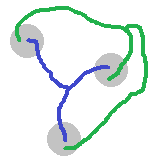
We’ll begin with a very well-known problem, which asks whether it’s possible for three houses on the plane to be connected to three utility suppliers without crossings.

utility

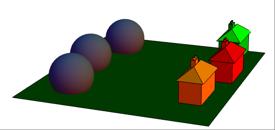
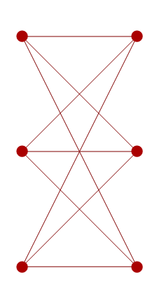
What appear to be three plutonium reactors are actually suppliers of electricity, water and gas, respectively. Ideally, we need to connect them with a planar arrangement of cables, aqueducts and pipes such that each of the three houses receive all three utilities. Proving that it’s impossible is not too difficult. Firstly, we reduce it to the graph-theoretic problem of trying to find a planar embedding of the complete bipartite graph K_3,3:

K33

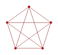
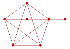
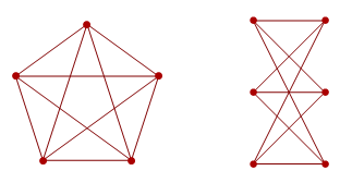
If we can find a planar embedding, all ‘faces’ created have an even number of edges, and therefore at least four edges. Plugging this inequality into Euler’s formula quickly leads to a contradiction, so there can be no such embedding. A related problem asks whether we can embed the complete graph K_5 into the plane; again, it is impossible by a similar argument. This problem might arise if you wanted to connect five houses in Edwin Abbott’s Flatland with telephone wires, long before the idea of a telephone exchange was invented.

K5

So, neither of these graphs are planar. Since K_5 is non-planar, the following graph doesn’t have a Tartarus-bound feline’s probability of being planar:

major

More generally, we obviously can’t make a graph less planar by performing any of the following operations:

  • Contracting edges (replacing two adjacent vertices with a single vertex connected to all of their neighbours);
  • Deleting edges (self-explanatory);
  • Deleting vertices (for simplicity, isolated vertices).

If we can do this to a graph G to obtain another graph G’, then G’ is said to be a graph minor of G. There’s a very deep and powerful theorem, the Robertson-Seymour theorem, which states that graphs form something called a well-quasi-order under the relation of graph-minorship.

So, what is a well-quasi-order?

I’m sure I’ve mentioned the fact that there is no infinite decreasing sequence of ordinals. Since the ordinals have a total order imposed on them, that is equivalent to the fact that in any infinite sequence {x_1, x_2, x_3, …}, there must be elements x_i and x_j such that both i < j and x_i < x_j. A well-quasi-order has the exact same definition, applied to a partial order such as graph-minorship.

So, we can’t have an infinite sequence of graphs, such that no graph is a minor of a later graph. We’ll use this later. For now, let’s consider the set of non-planar (finite!) graphs. This is a nice, big, countably infinite set with the property that if a graph has a minor in this set, then it must itself inhabit the set. This set contains things like K_3,3, K_5 and that graph we made by augmenting K_5.

Obviously, there’s a lot of redundancy here. We can get rid of the augmented K_5, since it’s not giving us any more information (we already know that K_5 is non-planar, which implies that the augmented K_5 is also non-planar). If our set of ‘forbidden minors’ is infinite, then at least one graph must be a minor of another, and we can remove the larger graph. So, by induction, the minimal set of forbidden minors must be finite. Indeed, there’s a theorem called Wagner’s theorem which states that this minimal set has just two elements: K_5 and K_3,3.

wagner

Any non-planar graph contains at least one of these as a minor. The best graph ever, the Petersen graph, actually features both of them as minors.

Linklessly embeddable graphs

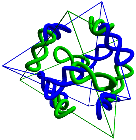
As well as planarity, we can consider other families of graphs closed under minorship. The Petersen graph is one of a set of seven forbidden minors for the property of linkless embedding. A graph is said to be linklessly embeddable if we can embed it into three-dimensional space such that no two cycles of vertices are linked. With the Petersen graph, we can’t. These seven forbidden minors include K_6 and are known collectively as the Petersen family (image courtesy of David Eppstein):

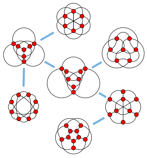
The light blue edges in the above graph of graphs represent Δ-Y transformations. These consist of replacing an induced 3-cycle with an induced star graph on 4 vertices, and are used for simplifying networks of resistors. The Petersen family shows that certain networks of resistors cannot be reduced by a suitable combination of Δ-Y transformations together with rules for resistances in series and parallel.

The set of graphs corresponding to reducible networks of resistors are closed under graph minorship, but the set of forbidden minors is far larger than the Petersen family. Yaming Yu demonstrated that this set contains at least 68 billion members.

Toroidal graphs

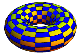
One way to ‘cheat’ at the water, gas and electricity problem is to place the houses and suppliers on the surface of a torus. Indeed, we can even have four houses and four utilities (e.g. water, gas, electricity and hydrogen) without any crossings. In particular, the graph K_4,4 is said to be toroidal. Similarly, the complete graph on seven vertices, K_7, is also toroidal (proof: seven-colour the hexagons in a honeycomb such that each hexagon is adjacent to hexagons of the six other colours, and such that the colouring is periodic in both dimensions). Whence, we obtain a brilliant polyhedron called the Szilassi polyhedron:

szilassi

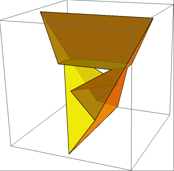
The Szilassi polyhedron has seven hexagonal faces, each of which neighbours the other six. We can convert this into the basic 7-couring of the hexagonal honeycomb by considering the universal cover of the Szilassi polyhedron. Informally, this is what we get when we unravel something to obtain a simply-connected space.

Even though we know that there is a finite set of forbidden minors for toroidal graphs, no-one has yet found one. This generalises to other surfaces as well as the plane and torus; examples include the Klein bottle, real projective plane and an infinitude of multi-holed tori.

Topological minors

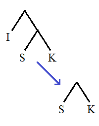
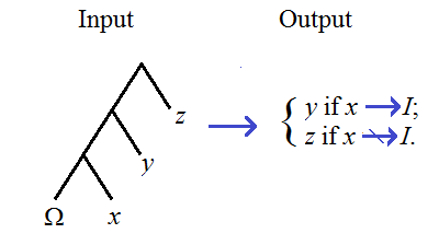
A related concept is that of a topological minor. All topological minors are graph minors, but not all graph minors are topological minors. A topological minor of a graph G is one which can be homeomorphically embedded into a subgraph of G by subdividing edges. I believe that an equivalent definition of topological minorship is to adapt the ordinary definition of graph minorship by replacing edge contractions with ‘double edge contractions’:

topological

In the diagram above, the lilac vertex has degree 2. The red vertices have arbitrary degree, being possibly connected to vertices not shown in the diagram.

It transpires that Wagner’s theorem holds when ‘graph minor’ is replaced with ‘topological minor’ (the name for this modified theorem is Kuratowski’s theorem), but the Robertson-Seymour theorem does not hold in general. Nevertheless, it does apply to the special cases of trees (the result, Kruskal’s tree theorem, implies that TREE(3) exists) and to graphs where every vertex has degree at most 3 (since under this restriction, topological minors and graph minors are equivalent).

Friedman’s SSCG function

Let’s concentrate on simple subcubic graphs, that is to say each vertex has degree at most 3. Harvey Friedman formulated a fast-growing function, SSCG, which is defined like tree() but with subcubic graphs instead of trees. In particular, SSCG(k) is the length of the longest sequence of simple subcubic graphs, such that no graph is a minor of a later graph, and the nth graph has at most k + n vertices.

Friedman commented that SSCG(13) is much larger than TREE(3); here I’ll improve the bound to show that even SSCG(3) is larger than TREE(TREE(…TREE(3)…)) with a shedload of nested applications of the TREE function.

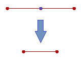
Note that there is no requirement that the graphs in question be connected. In the diagrams below, I’ll indicate the disjoint union of graphs with a plus (+) symbol, and the disjoint union of n identical graphs by preceding it with a number n. Firstly, the best lower bound I can attain for SSCG(2) is merely 3 × 2^(3 × 2^95) − 9 (i.e. less than a googolplex), which I conjecture is optimal.

SSCG2

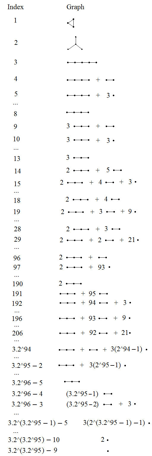
It’s not difficult to show that the first few moves must be optimal. After the first move, we’re restricted to forests, and the second move further restricts us to disjoint unions of line graphs. I proceeded using a greedy algorithm, ensuring that the corresponding ordinal (replace each line graph on n vertices with the ordinal ω^(n−1)) is as large as possible. Greedy algorithms often give optimal solutions to simple problems, although others (travelling salesman, for example) resist this approach.

SSCG(2) is quite small. If we want to beat TREE(3), we’re going to need at least SSCG(3). We’ll also need some way of encoding labelled trees as simple subcubic graphs. Since the nodes of the tree can have arbitrary degree, but the vertices of the subcubic graph have degree ≤ 3, it is insufficient to use individual vertices to represent nodes. Instead, we encode each node as a fused cycle and triangle. The labels will be acyclic trees of vertices, for simplicity.

TREE-node

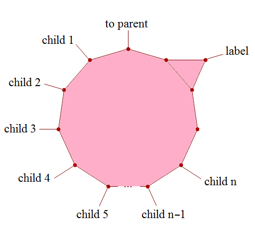
We connect these nodes together in the obvious way. For a tree to be a minor of another tree, it is obvious that nodes (pairs of connected cycles) must map to nodes, and that this corresponds to an inf- and label-preserving embedding. Actually, it is even more restrictive than that: the children must appear in the same order.

Each node has n + l + 6 vertices, where n is the number of children and l is the number of vertices in the label. We also need a distinguished ‘root’ node, designed so that it can only embed into the root of another tree. The root node is the only one where both cycles (triangles in this case) are eventually connected to other cycles.

root-node

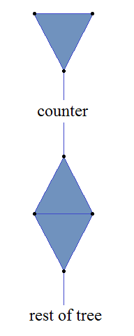
The root node doesn’t require a label. The size of the tree increases by up to l + 7 vertices for each step in the TREE sequence, so we need a ‘counter’ which decreases in length from l + 7 to 1 vertices between adjacent steps in the TREE sequence. This ensures that the nth graph doesn’t exceed its limit of n + k vertices.

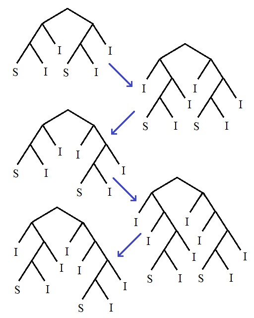
It’s easy to find a long sequence of graphs, which can take us up from 4 vertices to a large number of vertices, whilst not appearing as minors of any tree. Here’s how such a sequence might start:

first17

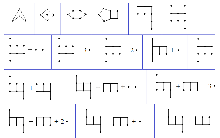
Note that the first two graphs are the forbidden minors for the set of outerplanar graphs (graphs which can be embedded on the plane so that all vertices are exposed). All subsequent graphs are outerplanar. The third graph has three fused cycles, and no subsequent graph has three fused cycles. All the following graphs contain a pair of fused 4-cycles, whereas the encodings of the labelled trees do not feature this as a minor.

After a while, subsequent graphs are a disjoint union of copies of the following ‘molecules’ together with the encoding of a labelled tree. The IUPAC identifiers for organic compounds are very useful for naming structures; James Aaronson and I designed a way of systematically naming polyominoes with a similar system.

molecules

Note that none of these appear as a minor of a later molecule, nor as a minor of an encoding of a labelled tree. Hence, as I mentioned earlier, we can create an extremely long sequence of TREE(TREE(TREE(…TREE(3)…))) graphs, with an incredible number of nested applications of the TREE function. Consequently, we have the nice tight bounds SSCG(2) « TREE(3) « SSCG(3), where « indicates ‘mind-bogglingly greater than’.

Strength of the Robertson-Seymour theorem

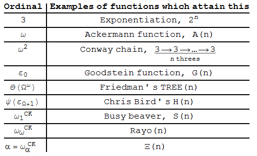
I’m not sure whether anyone has located the ordinal which measures the strength of the Robertson-Seymour theorem. It’s obviously at least the small Veblen ordinal (since it implies Kruskal’s tree theorem, and SSCG overtakes TREE), and strictly below the Church-Kleene ordinal (deciding whether a graph is a minor of another graph is recursively decidable).

Anyhow, the proof of the Robertson-Seymour theorem is very difficult and occupies several hundred pages.

Posted in Fast-growing functions, Uncategorized | 23 Comments

Alexandroff line

If this isn’t one of Ben Elliott and Hunter Spink’s bizarre mathematical objects of the week, it certainly deserves to be. This is a strange object which locally behaves like the real line, but is much longer. Instead of considering the entire real line, we’ll focus on the positive half-line:

real-line

As shown above, it’s obtained by gluing together a countable set of intervals. In the diagram above, they are indexed by the ordinal ω. If we do the same thing for the ordinal ω², then we obtain the same ordinary real half-line:

real-line2

The fusible numbers give a way of gluing together ε_0 intervals to obtain the real half-line. We can find similar constructions for all countable ordinals. Can we find an uncountable well-ordered subset X of the real line? The answer is no. For every x in X, there is a unique successor, S(x). Between x and S(x), there exists a rational number f(x). Clearly, the function f must be injective, so X is at most countably infinite.

So, what happens if we glue together ω_1 intervals, where ω_1 is the first uncountable ordinal? This must be longer than the real line, but for every point α, the interval [0,α) is homeomorphic to the real half-line [0,∞), which is in turn homeomorphic to the semi-open interval [0,1). Hence, we have something that locally resembles the real half-line, known as the Alexandroff ray. Gluing together two of these, back-to-back, gives the Alexandroff line, which locally resembles the real line despite being infinitely longer in both directions.

And guess what? In the Cartesian product (Alexandroff line)^2, we can pack uncountably many figure-eights. Can we pack as many figure-eights into the Alexandroff plane as we can circles? The answer, of course, is ‘if and only if the continuum hypothesis is true’…

Posted in Uncategorized | Leave a comment

Generalised Truchet tiles

A long time ago, in a monastery far away, a monk called Sebastian Truchet decided to create patterns by tiling a square grid with a single type of tile (in two orientations). For instance, one possible pattern of 64 Truchet tiles is shown below:

truchet2

There is a single non-trivial loop of length 12 on a background of trivial loops (henceforth referred to as ‘trivs’) of length 4. In general, we consider these patterns on an infinite grid of Truchet tiles, all but a finite portion of which is the lattice of trivs. To obtain this background pattern, colour the grid in a checkerboard fashion, where the colour of the square determines the orientation of the tile to place upon it.

We’ll then introduce some simple moves you can apply to a Truchet tiling to obtain another Truchet tiling. The simplest move is the Type 0A move, which enables a loop to expand by engulfing a triv. Alternatively, a loop can reduce its size by releasing a triv. The Type 0A move is depicted in this diagram:

type-0a

The actual tiles do not have colours; the red in the diagram above is for indication purposes only. A loop (a portion of which is visible in this 2 by 2 block, and shown in red) can either enlarge or shrink by swallowing or liberating the central triv. The reversibility of this process is indicated by the double-ended arrow, and will apply to all other moves as well.

Loops can expand and shrink, but non-trivial loops cannot join or split. They behave like phospholipid membranes, exhibiting endocytosis (swallowing trivs) and exocytosis (liberating trivs). In this analogy, the trivs resemble vesicles, small membrane-bound structures containing molecules.

A straightforward proof by induction can be used to show that any finite configuration of loops can be completely ‘evaporated’ into the background lattice of trivs. By reversibility, any configuration can spontaneously emerge. On a rather pointless side-note, all Truchet tiles can be 2-coloured and performing moves does not damage the consistency of the colouring. I’ve 2-coloured a random Truchet tiling below:

bicolour

A final observation is that the length of every loop must be divisible by 4. This is easy to prove, and I’ll leave it as an exercise to the reader.

Another tile

Things get more interesting when a second type of tile, the bridge, is added. This also has two distinct orientations, which differ by a rotation by ½π. Much more complicated structures can arise when the bridge is added, including knots and links:

truchet3

One particularly basic loop is a lemniscate, which cannot spontaneously evaporate under repeated application of the Type 0A rule. The two branches of the lemniscate can expand and contract, just like ordinary loops.

lemniscate

The behaviour is still uninteresting, since the lemniscate cannot drift along the board; the bridge is fixed as it cannot feature in a Type 0A move. Hence, it’s quite an unrealistic model of … whatever we’re supposed to be modelling. ANKOS meets string theory?

Hence, we’ll add a second move, Type 0B, which allows a bridge to move in space without affecting the topology of anything. The Type 0B move is depicted below:

type-0b

As usual, the colours are irrelevant and merely used to illustrate that the topology is preserved by this move. When the bridge is ‘shifted’ by one square, the orientation flips to obey parity constraints. So, lemniscates can now drift across the board as well as growing and shrinking. We now need to add another three moves, known as Reidemeister moves, to enable equivalent knots to transform into each other. Through a combinatorial and geometrical casebash, one can show that two knot diagrams can be interchanged if and only if the knots are equivalent.

type-123

Interestingly, the third of these diagrams is an ambigram — it is identical if you rotate the entire thing by π. Lemniscates can now unravel to give a self-avoiding loop, which can then evaporate into trivs. Equivalently, any unknot can appear from the quiescent background. However, non-trivial knots such as the trefoil cannot evaporate into trivs, nor fuse together, nor exhibit a whole manner of other unrealistic behaviour.

Knot invariants

Proving that the trefoil is not equivalent to the unknot took a surprising amount of time. The simplest knot invariant is tricolourability:

trefoil-tricolour

A knot diagram is tricolourable if you can colour the components of the knot such that:

  • At every bridge, the three components are either all the same colour or all different colours (c.f. the card game Set);
  • The knot is not all the same colour.

It’s very straightforward to show that the trefoil is tricolourable (see above), the triv is not, and Reidemeister moves preserve tricolourability. Hence, no unknot can be tricoloured, and thus the trefoil is not equivalent to the unknot.

Nowadays, knot invariants are much more sophisticated. Examples include the HOMFLY polynomial (named after six of its eight inventors), the Alexander polynomial and the Jones polynomial. It is an open problem as to whether the most advanced set of invariants, the Vassiliev invariants, can distinguish between any two knots.

Posted in Uncategorized | Leave a comment

Cipher 11: Musical mayhem

This cipher again is separated into two parts, namely an audio file and the following ciphertext.

ZKIGPWQ SLZSIIJ PBJRQKI TIMFTBE PEIVCNP
CVHFEHA OAXINDB PTGDPUO PSJRBEP ZAAAAAA

Unless you’re pitch perfect, you might also find this useful:

Print Carlotti

I’ll leave you to work out the significance of all this. Once again, the password for the secret area is purely lower-case.

Posted in Ciphers | Leave a comment

Bombers and Basilisks

Tim Hutton has announced the release of Ready 0.5, which is now able to support cellular automata and reaction-diffusion systems on three-dimensional honeycombs. There are a few sample patterns on Penrose tilings as well.

Replicators and Feynman diagrams

On the subject of cellular automata, Nathan Thompson discovered a variant of Conway’s Game of Life in 1994. It was termed ‘HighLife’ due to the existence of a small replicator, which copies itself every twelve generations. An early discovery was that the replicator can drag a blinker (cluster of three cells) behind it, translating itself by (8,8) every 48 generations:

The c/6 spaceship in HighLife

For a while, people were unsure what this spaceship should be called. David Bell had recently conceived his second child, Carina (named after the constellation), and there were proposals to name the spaceship after her. Eventually, however, the community settled upon the term ‘bomber’ to describe how it appears to periodically emit small explosions every 24 generations.

Rather than considering these things as two-dimensional clusters of cells changing over time, it is convenient to abstract away most of the details. The replicator and bomber then become very simple objects, which can be viewed as ‘Feynman diagrams’:

feynman-diagrams

Space and time are represented on the horizontal and vertical axes, respectively; as time progresses, one moves down the diagram. The Feynman diagram for the replicator is Pascal’s triangle modulo 2 (resembling the Sierpinski triangle), whilst the blinker pulled behind the bomber causes it to remain bounded instead of expanding forever. The replicator units killed by the blinker are represented by green dots in the diagram.

The bomber is said to travel at a speed of c/6, which means that (on average) it translates by one cell every 6 generations (timesteps). More precisely, its velocity is (8,8)c/48, as it travels 8 units up and 8 units to the left every 48 generations. This is clearly the fastest possible speed a replicator unit can move at, and is the speed at which an untamed replicator expands.

XOR-extendable spaceships

In 1999, Dean Hickerson wondered whether slower speeds are possible. In theory, a string of replicator units could push a blinker at one end and pull another at the other end. We already have a ‘pull’ reaction (the basic one performed by the bomber); a (5,3) push reaction was found by Dean Hickerson. This is described in the last paragraph of this article.

This would ordinarily be incompatible with the (8,8) pull reaction, since (5,3) isn’t the same vector as (8,8). Fortunately, a parallel replicator can subsequently push it by (3,5), for an overall displacement of (8,8). The Feynman diagram for the push reaction is much more complicated than the pull reaction:

push-reaction

Not much became of this idea. It was realised that such a beast would be colossal (estimated size: 2^60 replicator units), and the idea was abandoned. Occasionally, people talked about the possibility of one of these XOR-extendable spaceships, but no exhaustive searches were done.

Until now, that is. I’ve discovered the first XOR-extendable spaceship in HighLife, which I have named the Basilisk due to its length. Indeed, if printed on graph paper at the scale of one cell per millimetre, it would be long enough to reach the Moon!

Using some linear algebra, I realised that the most fruitful speed to search for was c/69. It’s not too slow, nor too fast, and most importantly the feedback polynomial (a term I’ll elaborate upon later in this article) has a sufficiently large order for me to be confident that c/69 XOR-extendable spaceships can exist. I decided that a good starting point would be to draw the Feynman diagram for the ‘head’ of this spaceship:

basilisk-head

The colour of each dot (white or black) is obtained by adding together the two dots above it, modulo 2. This operation of addition modulo 2 is also known as exclusive disjunction, symmetric difference or simply ‘XOR’. Note that the bottom row is identical to the top row, but shifted two dots (corresponding to (8,8) in the original cellular automaton) to the left. These constraints are sufficient to extend the pattern above ad infinitum.

We can do the same for the tail of the spaceship, shown below. The two green dots at the back end correspond to the standard pull reaction exhibited by the bomber spaceship. There are many possible tails, and I had to include all of them in my search program to ensure that a solution was found.

basilisk-tail

Ideally, we want these two diagrams to ‘match up’ somewhere, so that we can connect the head and tail. This is not easy, since it requires the top row to agree in 46 consecutive bits. It’s quite possible that the string of bits enters a periodic behaviour before a match is found; that’s why we need to search for matches with many potential tails.

It transpires that the string of bits can be generated by a linear feedback shift register. This is defined in a similar manner to the Fibonacci sequence, but where each term depends on the previous 46 terms, rather than the previous 2. Also, it is over the finite field F_2 instead of the integers. The behaviour is obviously cyclic, and a little linear algebra and trial-and-error shows that the period is precisely 987964849939.

Due to the huge number of head/tail pairings, a match occurs well before that. The completed spaceship is just under 85 billion replicator units long. Searching for this required the development of a super-optimised algorithm (several orders of magnitude faster than the naive approach) involving matrix exponentiation and a hash table. After a couple of hours of searching, it stumbled across four potential solutions in quick succession. The one which looked the most promising is shown below:

The completed Basilisk -- click to enlarge

The Feynman diagram of the Basilisk — click to enlarge

Obviously, I can’t generate an RLE file for the whole pattern. I have, however, produced a proof-of-concept pattern file, featuring an ellipsis to show where I’ve omitted over 84 billion replicator units. You can view and run this in Golly (it works for about 18000 generations before the omission catches up to the ends and destroys the spaceship; the complete Basilisk runs smoothly forever).

Since the proof-of-concept works, and I’ve confirmed by linear algebra that the head and tail do indeed match up, the existence of the Basilisk is rigorously proved.

Posted in Uncategorized | Leave a comment

The Ξ function

This is the final article on fast-growing functions. In the first two articles we looked at computable functions, up to and including Friedman’s TREE function. The third article described the Busy Beaver function, which eventually overtakes all computable functions. This article will explore oracle Turing machines, Rayo’s number and ultimately give a inconceivably fast-growing function Ξ, such that Ξ(10^6) far exceeds any number anyone has yet defined.

hierarchy2

Oracle Turing machines

The first approach to creating functions faster than the Busy Beaver was to equip a Turing machine with a special ‘oracle’, which it can consult to solve the halting problem. These ‘second-order Turing machines’ are more powerful than ordinary Turing machines. The equivalent of the Busy Beaver function for second-order machines, S_2(n), cannot be expressed as any computable sequence of applications of the ordinary Busy Beaver function S. As such, it must correspond to the third admissible ordinal, ω2CK.

There is no need to stop there; we can define third-order Turing machines and so on. The kth-order Busy Beaver function S_k gives us the ordinal ωkCK.

If we can represent Turing machines of arbitrary order in a specific notation, it’s possible to define a function with growth rate corresponding to the ordinal ωωCK. The most elegant approach, considered by Rayo, was to use first-order logic as an alternative to Turing machines.

First-order logic

In first-order logic, we have a set of symbols:

  • Basic arithmetic operators, namely + and ×.
  • Elementary natural numbers, 0 and 1.
  • Parentheses, ( and ).
  • Variables which can range over the natural numbers. We have an infinite alphabet of variables {a, b, c, d, …, z, a’, b’, c’, …, z’, a”, b”, …}, which can be reduced to a finite alphabet if we use ‘ (prime) as a separate symbol.
  • The binary operator x == y, which gives a Boolean value (true or false) depending on whether the naturals x and y are equal.
  • Basic logical operators, namely AND, OR and NOT. In principle, these can all be replaced with NAND.
  • The existential quantifier ∃ and the universal quantifier ∀, together with ‘such that’ (represented by the colon, ‘:’).

For instance, Lagrange’s four square theorem can be written as ∀n:(∃a:(∃b:(∃c:(∃d:((a×a)+(b×b)+(c×c)+(d×d) == n))))). The busy beaver function can be expressed in first-order logic, as can any of the higher-order busy beaver functions mentioned above.

Rayo’s function Rayo(n) is defined as ‘the largest integer expressible uniquely by n symbols in first-order logic’. It must necessarily be ωωCK, since it can be bounded above by the diagonal sequence of nth-order Busy Beaver functions, but dominates any fixed-order Busy Beaver function. Rayo used his function to define a very large number, Rayo(10^100), to win a competition. We’re now going to use a third model of computation, combinatory logic, to absolutely annihilate this record.

Combinatory logic

Combinatory logic uses the idea of combinators, which are functions mapping combinators to combinators. We usually use three primitive combinators, namely I (identity function), K and S. Applications of combinators can be represented as a binary tree, where the function is on the left and the argument is on the right. The ‘rules’ for applying I,K,S are displayed below:

SKI-calculus

The process of taking the leftmost combinator in a tree and applying the respective rule is known as beta reduction. Some things eventually β-reduce to give the identity combinator. An example of this is the following tree:

beta-reduction

Some trees do not reduce to the identity combinator. We say that this particular one has an output of size 2; this is the number of leaf nodes in the final stage of the β-reduction before it reaches a state where we can β-reduce no further.

beta-reduction2

And there are those which grow infinitely:

beta-reduction3

With these three combinators, it’s possible to emulate Turing machines. We can represent natural numbers with functions known as Church numerals and perform arithmetic and logical operations. Recursion and iteration are also possible in this system.

Generalised combinatory logic and the Ξ function

Trees of SKI combinators are no more powerful than Turing machines. Nevertheless, we can actually strengthen it considerably by introducing a new super-combinator, the oracle combinator Ω. This accepts three arguments, and returns the second argument if and only if the first argument β-reduces to I, and returns the third argument otherwise. Here is a visual depiction:

oracle-combinator

It’s possible to define paradoxical, nonsensical, self-referential statements. We’ll remove this contradiction by being careful and only concentrating on well-founded trees. Firstly, trees consisting entirely of S, K and I are called ‘rank 0’. If, in the sequence of beta-reductions of a tree T, we only have to apply Ω to trees of rank less than the ordinal α, then we say that T has rank α. Trees with ranks are known as well-founded, as the definition resembles that of a set obeying the axiom of foundation (and thereby inhabiting the von Neumann universe).

We can build a rank-2 tree capable of computing the Busy Beaver function. We can also build existential and universal quantifiers using the oracle combinator, so a n-quantified expression in first-order logic can be evaluated by a rank-(n+1) tree. Hence, using a rank-ω tree, we can compute Rayo’s function. It shouldn’t be too difficult to imagine this requiring far fewer than 10^6 combinators.

I define my function, Ξ(n) to give the size of the largest output of a well-founded tree of n combinators. Consequently, Ξ(10^6) is inconceivably larger than the largest number defined before, namely Rayo(10^100). If you look at the ordinal table at the top of the page, you’ll see how much faster Ξ is than Rayo’s function.

Beyond Ξ?

If you add another oracle combinator, Ω’, capable of testing whether an expression is well-founded, then we can compute the Ξ function and much more. The variant of Ξ defined for the combinatory logic defined using {S, K, I, Ω, Ω’} is called Ξ_2, and has an even faster growth rate. You can continue adding further oracle symbols to obtain even faster-growing functions. I’m not going to bother doing this, though, since it’s really quite pointless as we have already broken the record.

Posted in Fast-growing functions | 50 Comments

Topological tacks

If you’ve bought a box of drawing pins from a stationery store, you’ll observe that the pins do not pack tightly at all, and there is lots of empty space in there. Indeed, it’s impossible to pack them particularly efficiently, due to an interesting theorem in topology. We’ll begin by considering the old puzzle that asks whether we can fit uncountably many topological lemniscates in the plane. Here are some examples of topological lemniscates in the plane:

lemniscates

We can certainly get a countably infinite set of disjoint topological lemniscates, by nesting them inside each other, analogous to Russian dolls. After some initial thought, you can deduce that there are no uncountable sets of disjoint topological lemniscates; each ‘lobe’ must contain a rational point, so we can define a function from the set of lemniscates to the set Q² × Q² of ordered pairs of rational points by choosing an arbitrary point in each lobe. This function must be injective, as otherwise the lemniscates must intersect. There are only countably many ordered pairs of rational points, completing the proof.

A variant of this problem is whether there exists a set of uncountably many disjoint topological Y-shapes in the plane. This is strictly harder since a topological lemniscate is necessarily a superset of a topological Y-shape:

8impliesY

Again, the answer is still no. James Aaronson showed me an elegant proof, involving the non-planarity of the complete bipartite graph K3,3. We map each Y-shape to a triple of rational circles, each one of which contains precisely one of the three endpoints and does not contain the centre. This isn’t quite an injection, as two disjoint Y-shapes can map to the same triple of rational circles:

not-injective

However, three disjoint Y-shapes cannot map to the same triple of rational circles, as it would imply that the complete bipartite graph K3,3 is planar. It’s trivial to prove that this is false, with a little help from the Jordan Curve Theorem.

What about the surface of a torus? K3,3 is a toroidal graph (indeed, it’s possible to draw K7 on the torus without edges crossing), so the argument breaks down. It can be repaired, however, by covering the torus with a finite collection of overlapping simply-connected regions, each of which can only contain countably many topological Y-shapes.

torus-grid

In the example above, each region is a 2-by-2 block containing two blue and two yellow squares. The centre of every Y-shape must lie in the interior of at least one region (even if it lies on the boundary between two squares). We can apply this argument to any topological surface of finite genus to show that only countably many topological Y-shapes can inhabit it.

There is actually a generalisation to R^n. A tack is the union of a line segment and an open (n−1)-ball, which intersect at a single point (an endpoint of the line segment, which lies in the interior of the ball). It has been proved that there does not exist an uncountable set of disjoint topological tacks in R^n for any n. This implies that they can’t be packed tightly, which is why there is lots of empty space left over in the box of drawing pins.

Posted in Uncategorized | Leave a comment

Egmohedron

Partially inspired by the chiral icosahedral sculptures by George Hart and Bathsheba Grossman, I have decided to create one of my own. It’s composed of thirty identical components, each of which is a distorted lemniscate. Note that the lemniscate has a Klein 4-group of symmetries:

lemniscate

In principle, this could be constructed by slotting together two identical simply-connected halves, which can easily be produced by three-dimensional printing. This lemniscate can then be used as a ‘building block’ to assemble more complex configurations. For instance, the EGMO logo is composed of five of these lemniscates arranged in a symmetrical design:

egmo-logo

It’s possible to extend this five-fold symmetry to chiral icosahedral symmetry (order 60), producing an elaborate arrangement of linked lemniscates known as the egmohedron. Now that I’ve discovered how to create animations in Mathematica, I can’t resist doing this. Sorry if it eats up your bandwidth…

egmohedron

If I can gain access to a 3D printer, I’ll try building an actual egmohedron. The production costs should be relatively cheap due to being composed of one unique part, which should be easily printable. I might need to revise the shape of the lemniscate to ensure that the structure is rigid.

Assuming everything goes to plan and we can make sufficiently many egmohedra in the next couple of months, it might be possible to award them as prizes to the gold medallists in EGMO 2013. I can’t guarantee anything, of course.

Group actions

There are thirty lemniscates in total, partitioned into five sets (shown as different colours), each containing six lemniscates positioned at the vertices of an octahedron. If you consider the group action of the rotational group on these five sets, you’ll be able to observe the isomorphism IA5. The stabiliser of each set is the chiral tetrahedral group, isomorphic to A4. Skewering the lemniscates in a particular set gives a tetrahedron:

tetrahedra

If you skewer all thirty lemniscates in the manner shown above, you’ll obtain the famous compound of five tetrahedra. Assuming my memory serves me correctly, Joseph Myers has made a cardboard model of it.

Each lemniscate is trivially equivalent to the unknot. Any two ‘adjacent’ lemniscates form a Hopf link, shown clearly in the diagram of two tetrahedra.

Posted in Uncategorized | Leave a comment