In 1966, Norman Johnson completely classified all of the strictly convex polyhedra with regular polygonal faces. It is a remarkable fact, but not too difficult to prove, that there are precisely two infinite families (the prisms and antiprisms), together with a large but finite number (108) of exceptional objects.
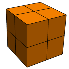
Firstly, by strictly convex, we mean that the shape is convex, and that no three vertices are collinear. Hence, we rule out possibilities such as this 24-faced cube:
To prove that there are no infinite families other than the prisms and antiprisms, we will first establish a lemma:
Lemma: If a strictly convex solid with regular faces has a face with 20 or more edges, then the solid is either a prism or antiprism.
Proof: We consider the possible vertex figures around each of the vertices of the n-gon (where  ). By angle constraints, we can narrow down the vertex figures to (n.3.3.3), (n.4.4) and (n.3.6). These are shown below:
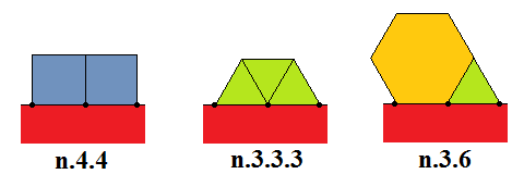
We can eliminate the n.3.6 configuration, by considering the other vertex where the triangle and hexagon meet. By the symmetry of the hexagon-triangle configuration, the only way to complete this is to add another n-gon; this would intersect the first n-gon, thereby rendering it invalid.
The n.4.4 and n.3.3.3 vertex configurations therefore automatically ‘induct’ to all vertices of the n-gon. This results in partial prisms and antiprisms, which (due to strict convexity) can only be completed by capping with another n-gon. This completes the proof of the lemma.
Theorem: There are only finitely many strictly convex solids with regular faces, other than the infinite families of prisms and antiprisms.
Proof: As there are only finitely many admissible faces (since 20-gons and higher are forbidden by the lemma), there are only finitely many possible vertex figures. Each one has a positive vertex angle defect (a discrete analogue to curvature), and the sum of the vertex angle defects must be 4π (known as Descartes’ theorem). This provides an upper bound for the number of vertices, which then upper-bounds the number of abstract polyhedra, and therefore the number of polyhedra (up to possible flexing). However, the rigidity theorem tells us that convex polyhedra cannot flex, completing the proof of the theorem.
The classification of finite strictly convex polyhedra with regular faces
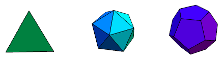
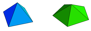
Now that we have two infinite families, it would be a good idea to look for other solids. The simplest are the remaining three Platonic solids (the cube and octahedron are a prism and antiprism, respectively).
As we know, we can also get another 13 Archimedean solids by modifying them with certain operations. It turns out that there are precisely 92 non-uniform strictly convex polyhedra with regular faces, known as Johnson solids. By analogy with the tetrahedron, we can also have a square pyramid (J1) and pentagonal pyramid (J2):
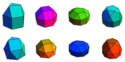
These can also be thought of as extremal mutilations of the octahedron and icosahedron, respectively. Similar processes can be applied to Archimedean solids, resulting in three cupolae and the pentagonal rotunda:
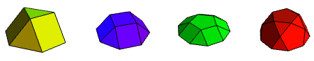
These are J3, J4, J5 and J6, respectively, in Johnson’s classification. Note that when we constructed the pentagonal pyramid, we did so by slicing an icosahedron. The remaining piece is a gyroelongated pentagonal pyramid (J11), which can itself be regarded as a union of a pentagonal pyramid and pentagonal prism. This opens up a whole new world of possibilities of joining pyramids to prisms and antiprisms (giving J7 to J11, inclusive):
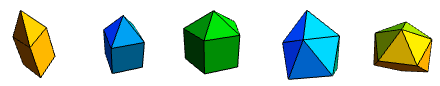
The octahedron is essentially two square pyramids, fused at their bases. The icosahedron is two pentagonal pyramids, connected by a pentagonal antiprism. We can repeat these types of constructions with other pyramids, yielding another six Johnson solids (J12 through to J17):
J7 through to J11 were constructed by elongating/gyroelongating pyramids. This can also be applied to the cupolae and pentagonal rotunda, yielding J12 to J25, inclusive.
In each case, the elongated form is displayed directly above the gyroelongated form. I’m not sure that I can easily motivate the next solid in the classification, which is a combination of two triangular prisms, meeting at a square face. It does have the very imaginative name, gyrobifastigium (J26), considering how simple and banal it is.
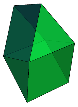
The most interesting thing about the gyrobifastigium is its etymology. The prefix bi- is obviously due to the fact that there are two triangular prisms. The gyro- describes how one is rotated with respect to the other, as opposed to having bilateral symmetry in the plane where they meet. But fastigium? Apparently, it is the Latin word for a summit, peak, or apexed roof.
Let’s return to the systematic construction of more Johnson polyhedra. J12 and J13 were built out of two pyramids, base-to-base. Replacing ‘pyramid’ with ‘cupola’ or ‘rotunda’ gives another eight Johnson solids (J27 to J34):
These, as with the other Johnson solids, have very systematic names such as triangular orthobicupola and pentagonal gyrocuploarotunda. Recall that J14 to J17 simply involved introducing interstitial prisms and antiprisms to the bipyramids; this trick also works here to give some more solids. Firstly, for the triangular bicupolae, we obtain elongated forms:
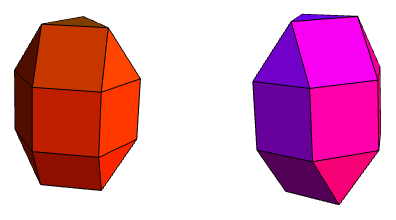
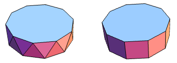
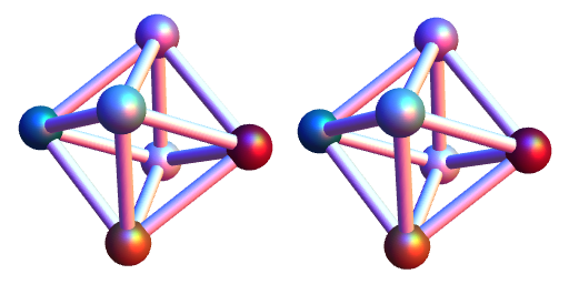
If we repeat for the square cupola, we only get one new form. The elongated square orthobicupola is just a rhombicuboctahedron (an Archimedean solid). By comparison, the elongated square gyrobicupola (J37) is an evil impostor, which has the same circumradius, inradius, midradius and volume as the rhombicuboctahedron, as well as the same quantities of each of the different faces, and even the same vertex figures on every vertex. More remarkably, it can even be shown that they have the same inertia tensor.
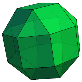
To an untrained observer, they look very similar, and you may even be able to convince multiple people for several hours that they are, in fact, looking at a rhombicuboctahedron. Sooner or later, however, people will start to suspect that it is merely a very convincing lookalike, noticing slight problems such as lack of vertex-transitivity, and the fact that it only has one equator of eight squares, rather than three.
Shown above are six elongated pentagonal forms. There are also five gyroelongated forms, shown below:
New polyhedra from old
We’re now just over halfway through the classification of Johnson solids. The next big idea is to erect pyramids on the faces of existing solids to produce new forms. Again, we’ll start with prisms, yielding another nine solids (J49 to J57):
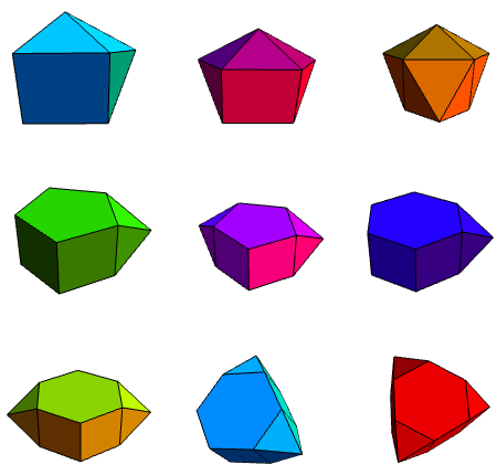
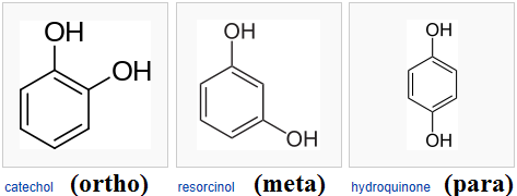
Johnson refers to pyramid erection as augmentation. Consequently, the top three solids are the augmented, biaugmented and triaugmented triangular prisms (J49, J50 and J51, respectively). Similarly, we get augmented and biaugmented pentagonal prisms (J52 and J53), and an augmented hexagonal prism (J54). However, both J56 and J57 could be called biagumented hexagonal prisms, so we need a way to distinguish between them. Johnson decided to borrow terminology from organic chemistry, used to describe the relative positions of functional groups on a benzene ring:
This terminology also comes in handy for dodecahedra. We have augmented, parabiaugmented, metabiaugmented and triaugmented dodecahedra (J58 to J61):
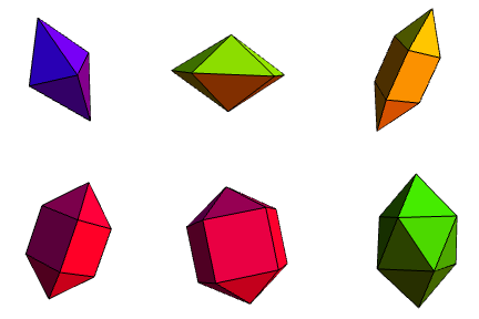
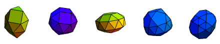
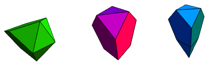
The reverse operation to augmentation is diminshing. The diminished and parabidiminshed icosahedra are the gyroelongated pentagonal pyramid and pentagonal antiprism, respectively. However, the metabidiminished icosahedron (J62) and tridiminished icosahedron (J63) are genuinely new forms. Adjacent to the three pentagonal faces of J63 is a triangular face, which can (only just!) accept an erected tetrahedron, giving an augmented tridiminshed icosahedron (J64). These three solids are shown below:
The next few solids are obtained by augmenting truncated regular solids not with pyramids, but with cupolae.
Again, their dodecahedral counterparts require prefixes to distinguish between the two biaugmented truncated dodecahedra.
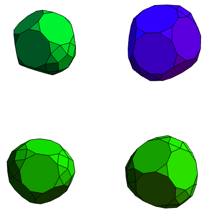
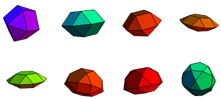
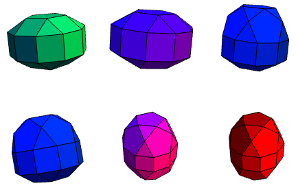
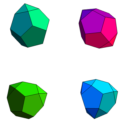
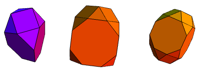
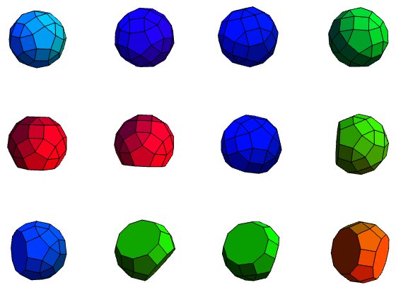
The next set of Johnson solids comes from modifying the rhombicosidodecahedron. In the same way that we can obtain the elongated square gyrobicupola (J37) by rotating a cupola of a rhombicuboctahedron, we can also gyrate the rhombicosidodecahedron. Additionally, it is possible to diminish it (by removing a cupola completely), or even perform different operations to different cupolae. Twelve new solids (J72 to J83) arise in this manner:
The top four are quite difficult to differentiate from each other. A systematic way is to look for pentagons and triangles sharing faces (there will be adjacent squares, which are easier to spot, nearby), to highlight the triangle, and to highlight pentagons which five highlighted triangles ‘point to’. Then, the highlighted pentagons correspond to gyrated cupolae.
Finally, there are nine additional Johnson solids (increasing the total to 92), which are ‘primitive’ and cannot be derived from modifying existing solids.
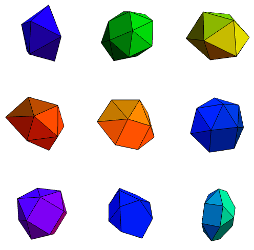
The first of these is called a snub disphenoid, which is a rather stupid name since snubbing a disphenoid would produce a polyhedron abstractly equivalent to a snub tetrahedron, i.e. an (irregular) icosahedron. Again, we have some interesting names, such as hebesphenomegacorona (J89) and disphenocingulum (J90).
And now you’ve seen them all.

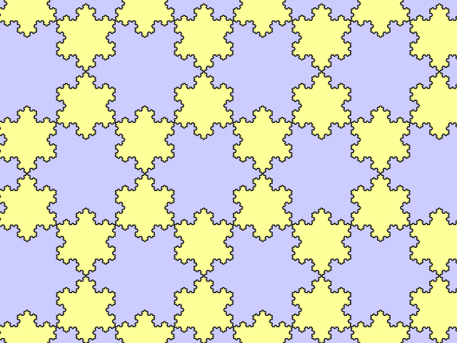
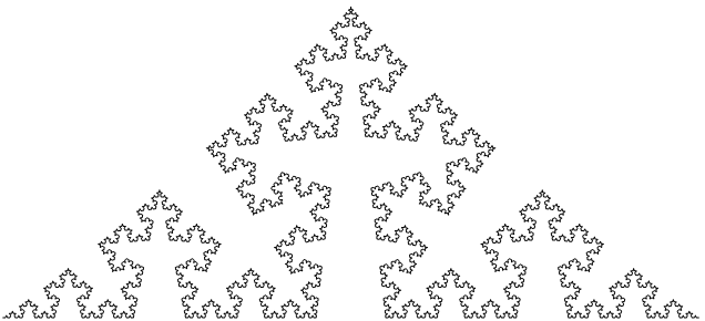
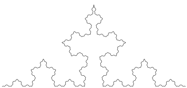
 . Varying the value of σ between ¼ and ½ yields a family of fractal curves, with Hausdorff dimension ranging from 1 (a straight line) to 2 (a spacefilling curve):
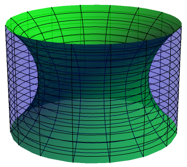
 about the z-axis; this can be demonstrated by the calculus of variations.

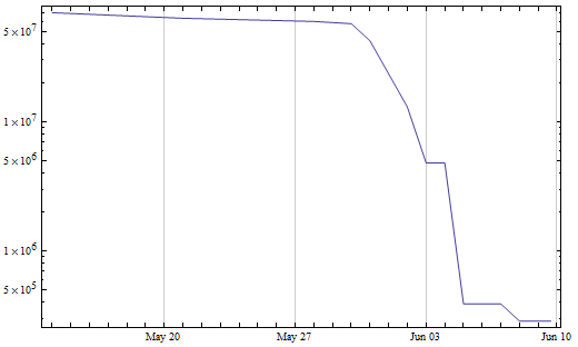
 disjoint from S. At the moment, there is an established upper bound of 26024 and a conditional result by Terry Tao et al claiming that
  . Reducing the value of k0 leads to a smaller value of:
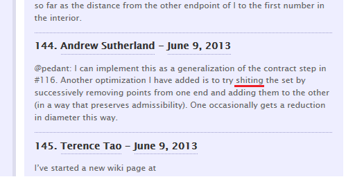
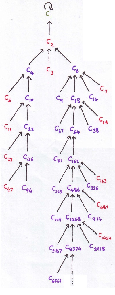
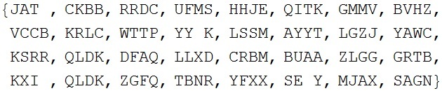
 with vertex set
  ; the edge set is
  , and for
  if and only if in the binary expansion of
  , the digit
  from the right is 1. So, for example,
  for odd
  and
and  for
for  or
or  .
. , there exists a vertex
  such that
  and
and  with
with  . The proof is constructive: let
  where
where  for
for  .
. with
with  countable is an induced subgraph of
  , we require an injective function
  with
with 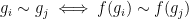 . Let
. Let  as a base case, with the inductive hypothesis that
  defined on
  obeys the rule. Then for the inductive step we can find
  adjacent to precisely the correct vertices due to the extension property.
 be two rival countable graphs with the extension property, and finding
  . Then supposing inductively that
  , and
, and  is defined on
  , we set values for
  and
and  using the extension property if they haven’t already been set. Hence
  . We can also start with an isomorphism between any two induced subgraphs of
  is obtained from
  . This is a corollary of uniqueness; it is very easy to show that
  ).
). is partitioned into finitely many subsets
  then at least one of the corresponding induced subgraphs is isomorphic to
  and
and  , suppose
  such that every
  is in
is in  , there is an
  , and
, and  , so
, so  , so in the general case, for some
  .
. for the same reason as above.
 and we go through each pair of vertices, constructing an edge between them with probability
  . The graph we get, independent of
  and
and  , and some vertex
  and
and  vertices is in fact the not-very-random-at-all graph.
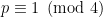 . Put
. Put 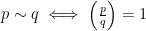 . To verify this you need to understand the basics of quadratic reciprocity and Dirichlet’s theorem.
 be universal; that is, writing
  and put
  . This one can be proved without any further knowledge.
 as a counterexample, your solution will be met not with awe or respect, but with disappointment and embarrassment. The same goes for any exams; if a well-known counterexample exists, the hypothesis is unlikely to be set as a question, whereas it’s not unlikely that the Rado graph should provide a counterexample.