Complex Projective 4-Space

The Not-Very-Random-At-All Graph

Posted on June 6, 2013 by ggendler

This is a guest post by Gabriel Gendler. As such, any views expressed in this post do not reflect the views of Complex Projective 4-Space or of Adam P. Goucher.

In a recent post Adam P. Goucher recommended that readers adopt the Petersen graph as their favourite graph, if they had not chosen one already. This post is designed to promote an alternative favourite graph – the Rado graph.

Definition

We start with the following, seemingly tame, definition. Define the countably infinite graph $R$ with vertex set $V(R) = v_0, v_1, v_2 \ldots$ ; the edge set is $E(R)$ , and for $i<j, (v_i, v_j) \in E(R)$ if and only if in the binary expansion of $j$ , the digit $i$ from the right is 1. So, for example, $v_0 \sim v_k$ for odd $k$ and $v_1 \sim v_k$ for $k \equiv 2$ or $3 \pmod 4$ .

The extension property

First, we observe a useful but not immediately interesting property: for any finite disjoint sets of vertices $V, W \in V(R)$ , there exists a vertex $x \notin V \bigcup W$ such that $x \sim v \forall v \in V$ and $\nexists w \in W$ with $x \sim w$ . The proof is constructive: let $x = v_t$ where $t = k \cdot 2^j + \sum_{v_i \in V} 2^i$ for $k$ and large enough $j$ both in $\mathbb{N}$ .

Induced subgraphs

Now we get our first impressive result. Every graph $G$ with $V(G)$ countable is an induced subgraph of $R$ . For, supposing the vertices of $G$ are labelled $g_0, g_1, g_2 \ldots$ , we require an injective function $f: V(G) \mapsto V(R)$ with $g_i \sim g_j \iff f(g_i) \sim f(g_j)$ . Let $f(g_0) = v_0$ as a base case, with the inductive hypothesis that $f$ defined on $g_0 \ldots g_n$ obeys the rule. Then for the inductive step we can find $f(g_{n+1}) \in R$ adjacent to precisely the correct vertices due to the extension property.

Uniqueness

Next things start to get weird, because it turns out that all countable graphs with the extension property are isomorphic. We will prove this by letting $R$ and $S$ be two rival countable graphs with the extension property, and finding $f$ an isomorphism between them. We label the vertices of $R$ and $S$ in the normal way and let $f(r_0) = s_0$ . Then supposing inductively that $f$ is legal and defined on $r_0 \ldots r_n$ , and $f^{-1}$ is defined on $s_0 \ldots s_n$ , we set values for $f(r_{n+1})$ and $f^{-1}(s_{n+1})$ using the extension property if they haven’t already been set. Hence $R \cong S$ . We can also start with an isomorphism between any two induced subgraphs of $R$ and build up the full isomorphism from there, so we find that the graph is symmetric and ultrahomogeneous.

That was quite momentous. You may have seen it coming, but just like global warming that doesn’t stop this from being a big deal. As a consequence the weirdness becomes endemic.

Damaging the graph

Suppose $R'$ is obtained from $R$ by deleting finitely many vertices and adding or deleting finitely many edges. Then $R \cong R'$ . This is a corollary of uniqueness; it is very easy to show that $R'$ has the extension property (notice that in the proof of the extension property $k$ can be any integer so there are infinitely many legal $x$ ).

That’s really weird. If the graph is subjected to GBH (or indeed initiated into a Cambridge drinking society) it retains its shape.

Tearing the graph into pieces

Equally weird is the following: If $V(R)$ is partitioned into finitely many subsets $A_1, A_2, A_3 \ldots$ then at least one of the corresponding induced subgraphs is isomorphic to $R$ . This follows immediately from the case of a partition into two sets. For sets $A$ and $B$ , suppose $A$ is not the Rado Graph. Then there are subsets $V_1, W_1 \subset A$ such that every $x$ extending $V_1, W_1$ is in $B$ . Now for any subsets $V_2, W_2 \subset B$ , there is an $x$ that extends $V_1 \bigcup V_2, W_1 \bigcup W_2$ , and $x \in B$ , so $B$ has the extension property. Hence either $A$ or $B \cong R$ , so in the general case, for some $k$ , $A_k \cong R$ .

Similarly, if the edges are $k$ -coloured for finite $k$ , then there exists an induced subgraph which is a 2-coloured Rado graph. The proof of this makes up the better part of a paper by Sauer and Pouzet which costs £30, so I won’t reproduce it here. However I will point out that this only needs to be proved for $k=3$ for the same reason as above.

The Random Graph

Perhaps you’re sufficiently weirded out already. Perhaps you’ve found all the weirdness so far rather run-of-the-mill. Either way, I think you’ll agree that the next realisation is about as weird as they come.

We start with an empty, countably infinite graph. We pick any $0 < p < 1$ and we go through each pair of vertices, constructing an edge between them with probability $p$ . The graph we get, independent of $p$ , is almost always (i.e. with probability 1) the Rado graph. This is actually easy to prove, using extension and uniqueness; for any set of vertices $V$ and $W$ , and some vertex $x$ not in $V$ or $W$ , the probability that $x \sim v \forall v \in V$ but $\nexists w \in W$ with $x \sim w$ is positive, so taken over all possible $x$ it is true with probability 1. Since $U$ and $V$ are finite, the number of pairs of subsets is countable, and the intersection of countably many events each with probability 1 is 1, as required.

At this point, the weirdness is so intense that it threatens to destroy the universe as we know it. Things fall apart at the seams. It turns out that the moon is made of cheese; China withdraws unilaterally from Tibet and voluntarily cedes all authority to Taipei. The Israeli government and the Palestinian Authority sign a peace treaty implementing a one-state solution, and the new country is known as the Federal Republic of Integral Bananas. Americans vote unilaterally to ban the ownership of firearms in a referendum, and scientists discover a cure for cancer whose active ingredient is powdered chocolate. Finally, every member of the IMO team gives up maths and enrols at Oxford for an undergraduate degree in History of Art. Why? Because the random graph on $\aleph_0$ vertices is in fact the not-very-random-at-all graph.

Alternative Constructions

Now that the Rado graph has ripped the universe apart it can sit back and just show off for a bit. Here are two alternative constructions of $R$ ; both can be verified using the extension property and are set as an exercise for the reader.

Let the vertex set be all primes $p \equiv 1 \pmod 4$ . Put $p \sim q \iff \left(\frac{p}{q}\right) = 1$ . To verify this you need to understand the basics of quadratic reciprocity and Dirichlet’s theorem.
Let $S \subset \mathbb{N}$ be universal; that is, writing $S$ as a string of 0s and 1s in the natural way, every finite string of 0s and 1s can be found in $S$ . Then let the vertex set be $\mathbb{Z}$ and put $a \sim b \iff |a-b| \in S$ . This one can be proved without any further knowledge.

Proving stuff about this graph is quite easy

Everything we’ve seen has been quite easy to prove. That’s what I like about the Rado graph; the definition is such that everything else just falls into place. To convince yourself of this, why not find a few simple properties of the Rado graph, such as its chromatic number, its diameter and its complement? Does there exist a Hamiltonian path through every vertex? In a cops and robbers game where the robber takes it in turns with n cops to move to an adjacent vertex (all the cops move at once), who wins? Everything seems to come straight out of the definition of the Rado graph.

Why you should adopt the Rado graph as your favourite graph

A favourite graph is most useful for testing hypotheses. As such, the Rado graph is an excellent choice of favourite graph because of three features that make it a good candidate for answering hypotheses in the negative. These are:

It is easy to work with. The immense symmetry, the extension property, the subgraph property and the uniqueness of the Rado graph make it very easy to prove things about it. Therefore it will ordinarily be easy to check whether a hypothesis is true for the Rado graph (see previous paragraph).
It has strange properties. This makes it feasible that the Rado graph should provide a much better answer to a problem than any other graph.
It is unusual. Suppose you were to bump into your friends as they struggle to prove or disprove some graph-theoretic hypothesis, and the Rado graph provides a counterexample. You can look forward to several minutes of sincere respect for such an elegant yet obscure solution. On the other hand, if your favourite graph is the complete graph on three vertices, and that provides a counterexample, then it’s probable that your friends will already have answered their hypothesis by the time you arrive. Moreover, if you are in time to use $K3$ as a counterexample, your solution will be met not with awe or respect, but with disappointment and embarrassment. The same goes for any exams; if a well-known counterexample exists, the hypothesis is unlikely to be set as a question, whereas it’s not unlikely that the Rado graph should provide a counterexample.

“But I’ve already got a favourite graph!”

I recognise that many people are already in a relationship with a graph, especially since those who were single a few weeks ago probably hooked up with the Petersen graph after being introduced to it by Adam. Nevertheless there are likely to be readers without one, either because they had a bad first date with the Petersen graph, or because they have broken up since then due to the inevitable disappointing relationship that followed those dream-like first few moments. Additionally, it’s probable that some readers didn’t see that post, in which case they might still be virgins. Finally, those in a relationship with the Petersen graph might be ready to move on; indeed, it is rather promiscuous (by which I mean overused), and just as any partner ought not to sleep around, so a favourite graph ought to be unusual. If, on the other hand, you are happily married to the Petersen graph, perhaps you might want to adopt the Rado graph as your favourite infinite graph. If the Petersen graph is insulted, remind it that the Rado graph contains infinitely many copies of the Petersen graph.

Sources

http://www.math.unt.edu/~mpc0061/logicgroup/randomgraph.pdf
http://en.wikipedia.org/wiki/Rado_graph
http://mabit.org.hu/~p_erdos/1963-04.pdf

Posted in Uncategorized | 10 Comments

Integral banana

Posted on June 5, 2013 by apgoucher

I have received numerous complaints (from the same person) that some of the content on cp4space is completely ridiculous. Of course, posting more serious mathematics would not solve the issue, since it would not alter the fact that, on cp4space, there are already several ridiculous posts. Hence, the only logical alternative is to make those ridiculous posts appear comparatively serious, by instead writing a single article of unparalleled silliness.

So, it occurred to me to mention a rather intriguing discovery I made. Usually, mathematical discoveries take a long period of dedication, since all of the low-hanging fruit has already been claimed by previous mathematicians. This, however, is something of an exception.

The banana was originally considered a rather exotic fruit (c.f. this video), but over time it has become accepted as being mundane and banal, no qualitatively different from the more indigenous apples and pears that have a habit of hitting unexpectant Trinity mathematicians. It is renowned for having a constant positive curvature and zero torsion. Hence, you can imagine my surprise when I encountered a banana with a point of inflection:

Yes, it’s a banana shaped like an integral sign. This is definitely noteworthy, since it opens up a whole world of new possibilities. After suitably resizing, it was not too difficult to state the divergence theroem using this more colourful substitute for the integral sign:

See how the equation suddenly comes to life? How much better it looks than the boring LaTeX-rendered \int symbol? How you’ve been spending years without realising the potential for fruit to feature in practically every piece of applied mathematics you perform?

Well, you have no excuse now. Here are some icons corresponding to the possible variants of the integral sign, together with the equivalent LaTeX commands:

$latex-equivalents$

We can use the divergence theorem, for instance, to prove the uniqueness of a solution to Poisson’s equation subject to a Dirichlet boundary condition.

As you can imagine, there is no limit to the amount of enjoyment you can derive from banana integrals. In fact, if you determine the conditions for existence and uniqueness of solutions to the Navier-Stokes equations, then you could even win $1000000 from the Clay Mathematics Institute and have fun at the same time!

Posted in Activities | 14 Comments

Iterated automorphism groups

Posted on June 3, 2013 by apgoucher

This was inspired by a discussion with James Aaronson outside the Chapel. We were contemplating group theory and automorphisms (specifically, trying to determine whether there exists a group of size strictly larger than $2^{\aleph_0}$ with only two automorphisms), and eventually considered the following question:

What happens if you begin with a group G, and iteratively apply the ‘automorphism group’ operator?

For a cyclic group of order n, where n has primitive roots, the automorphism group is the cyclic group of order φ(n). If a group is non-Abelian, its automorphism group is also non-Abelian (consider automorphisms arising from conjugation by elements which do not commute). Similarly, if a group is Abelian and non-cyclic, its automorphism group is non-Abelian. Hence, the groups that eventually reduce to the trivial group under repeated application of Aut are cyclic groups of order n such that {n, φ(n), φ(φ(n)), …, 1} all have primitive roots. James Aaronson completely characterised the integers with this property:

$3^n$ , for all $n \in \mathbb{N}$ ;
$2 \times 3^n$ ;
Primes p of the form $p = 2 \times 3^n + 1$ ;
2p, where p is a prime of that form;
4, 5, 10, 11, 22, 23, 46, 47 and 94.

These form the sequence A117729.

The next case is C8, which has no primitive roots. Its automorphism group is the Klein 4-group, C2 × C2. Since it is the additive group of a vector space over F2, the automorphism group is the group of linear maps (2 × 2 invertible matrices over F2 with linearly independent columns). It is not too hard to show that this is isomorphic to S3 (symmetric group with 6 elements), and that the direct sum $C_p^n$ has the general linear group GL(n, p) as its automorphism group.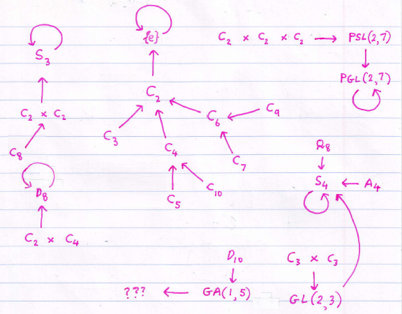

Most symmetric groups (the exceptions being n = 2 and n = 6) are their own automorphism groups. The next few cases, such as D8 and Q8, are included in the diagram below:

As the size of the group increases, these become difficult to compute.

For simple non-Abelian groups, the automorphism group is complete (equal to its own automorphism group). This is proved here. More generally, for centreless groups, it is possible to define a limit of a sequence of iterated automorphism groups, known as an automorphism tower. It has been proved that this process eventually terminates at some ordinal (not necessarily finite).

This is discussed in further detail on Math Overflow.

Posted in Uncategorized | 4 Comments

IMO team unveiled

Posted on May 29, 2013 by apgoucher

IMO team unveiled

After four long exams on contiguous days, the UKMT has selected the IMO team (some of whom are regular readers of this website). For the first time in history, this happens to be identical to the RMM team. Naturally, I congratulate the six team members for reaching this stage, and wish them the best of luck in the competition.

Posted in Uncategorized | 1 Comment

Pairwise versus overall

Posted on May 28, 2013 by apgoucher

A recurring general theme in mathematics is of a property being true of three objects when considered pairwise, but not true of the entire set. For example, earlier we considered non-trivial mutual friends, and how a simple graph is not sufficient to contain all information about the relationships between elements of a set. Here are a few more examples:

Coprimality

The integers 6, 10 and 15 are coprime, but any pair of them share a common factor. Consequently, the Diophantine equation $a^6 + b^{10} = c^{15}$ cannot be solved by the Sam Cappleman-Lynes technique, nor can it be disproved by Fermat’s Last Theorem.

In the statements of Beal’s conjecture, Fermat-Catalan conjecture and the abc conjecture (proof still unverified at the time of writing, since precisely one person understands inter-universal Teichmüller theory.) it doesn’t matter whether we use coprimality or pairwise coprimality, since the relation between the variables causes the notions to coincide.

Probabilities

If an ordered triple of random variables (x, y, z) can take the values (0, 0, 0), (1, 1, 0), (1, 0, 1) and (0, 1, 1) with equal probability, then any pair of variables are independent, but the third is determined entirely by those two. A similar situation occurs in three-particle quantum entanglement, where the total parity of the electron spins is restricted by conservation laws.

Food incompatibility triad

George Hart (geometer, and co-creator of Vi Hart) proposed the following problem:

Find three foods, such that any two are compatible, but the three together are incompatible.

This has been fiercely debated in the comments section of an article in the Guardian column of Alex Bellos. There doesn’t seem to be any generally accepted solution (Feynman erroneously claimed that {milk, tea, lemon} was a solution, but this is broken by the incompatibility of milk and lemon), and little progress has occurred since George Hart closed the question on the basis of it being too subjective.

Until now, that is. John Howe, Cameron Ford et al claim the following solution:

Pancakes
Lemon liqueur
Beef

The first two constitute a crêpe suzette, and the other two combinations apparently exist on the Internet, whereas their union does not. The solution has apparently been sent to George Hart, and I am unaware whether a response has been received. This may finally put to rest an age-old puzzle believed to have originated with the philosopher Wilfrid Sellars.

Posted in Uncategorized | Leave a comment

The Universe

Posted on May 26, 2013 by apgoucher

Some people have recently been discussing Eric Weinstein*, who has proposed a 14-dimensional theory of everything known as Geometric Unity. The media attention is possibly as a result of the trivial difference between his surname and that of the patent office clerk responsible for formulating general relativity.

* Not to be confused with Eric Weisstein, who created Wolfram MathWorld.

Whilst these theories of everything are concerned with the local field equations and particles at the most minute of scales, the large-scale structure of the universe is also very interesting and equally unknown. Here we’ll examine a few suggested candidates for the shape of the universe:

Curvature of space

When you gaze off into the depths of space, it is natural to imagine space as being $\mathbb{R}^3$ , an infinite Euclidean space. This is not, however, the only possibility. Space is locally curved (c.f. general relativity), and it has been suggested that it may in fact be globally curved. A constant positive Gaussian curvature would cause the universe to ‘curl up’ into a 3-sphere, whereas a negative Gaussian curvature corresponds to hyperbolic space.

Thanks to Gauss’s Theorem Egregium, it is possible to determine the local curvature by measuring distances in the propinquity of a point. Hence, it is theoretically possible to calculate the radius of the Earth by measuring distances between (four) cities. I tried this and computed a Cayley-Menger determinant; it differed from zero, proving that the Earth is not flat.

Cosmologists have measured the curvature of the universe to be within experimental error of zero, suggesting that (on a large scale) space is Euclidean. If space is indeed everywhere flat, this precludes the possibility of the universe being a 3-sphere. There are, however, several possible shapes, even with this restriction. Conway calls these platycosms.

Platycosms in two and three dimensions

In two dimensions, there are precisely two finite flat manifolds, the torus and Klein bottle. They differ in that one is an orientable surface, whereas the other is not. If we lived on a three-dimensional analogue of a Klein bottle, it would be possible to place a left-handed seashell on a spaceship, send it around the universe, and observe that it returns as a right-handed seashell.

There are ten finite three-dimensional platycosms (mentioned here), which are all feasible candidates for the shape of our universe. Other possibilities include an infinite universe (such as the Cartesian product of a circle and an infinite plane). I’m assuming that the universe doesn’t have a boundary, as this would be really weird.

Poincare dodecahedral space

Certain manifolds can be constructed by taking a simply-connected patch and identifying parts of its boundary. For example, a torus can be produced by identifying opposite edges of the unit square. A more complicated example is obtained by identifying opposite faces of a regular dodecahedron. 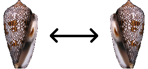Depending on how much you twist each face (by 36°, 108° or 180°), you can obtain different spaces (namely a Poincaré homology sphere, the Siefert-Weber space, and $\mathbb{RP}^3$ , respectively).

Based on data from the WMAP probe, some scientists conjecture that the shape of the universe is a Poincaré homology sphere. The evidence isn’t conclusive, however…

Posted in Uncategorized | 2 Comments

Sierpinski triangle

Posted on May 23, 2013 by apgoucher

The Sierpinski triangle is a surprisingly ubiquitous mathematical object. Rather than describing what a Sierpinski triangle is, I may as well show you a picture of one.

Essentially, it consists of three identical copies of itself, scaled by a factor of ½. This means that any reasonable definition (e.g. Hausdorff) gives the dimension of the Sierpinski triangle as $\dfrac{\log{3}}{\log{2}}$ . We can ask more detailed quantitative questions about the Sierpinski triangle:

Moment of inertia

This is quite an easy one, actually. If a Sierpinski triangle of mass m and side length l is rotated about an axis passing normally through its centre, dimensional analysis shows that the moment of inertia is given by $k m l^2$ for some dimensionless quantity k.

Using the recursive definition of the Sierpinski triangle and invoking the Huygens-Steiner theorem (you may know this as the parallel-axis theorem), we get a relation which can then be rearranged to give $k = \frac{1}{9}$ . So, the moment of inertia is simply $I = \frac{1}{9} ml^2$ .

From this, it is trivial to find the average squared distance between two points: $\frac{2}{9} l^2$ , also by Huygens-Steiner.

Mean distance

Finding the mean (unsquared) distance between two randomly-chosen points is much more non-trivial, and the result is due to Andreas Hanz. It transpires that the mean distance is $\dfrac{466}{885} l$ , and the variance of the distance is $904808318/14448151575 l^2$ . These results were determined by taking the limit (as the number of discs tends to infinity) of the (normalised) mean distance between two randomly chosen configurations in Tower of Hanoi puzzle.

Sierpinski tetrahedron

This is an obvious generalisation of the Sierpinski triangle. It is, however, easier to construct: Let x,y,z be real numbers (which are not dyadic rationals) in the interval [0,1]. Then, (x,y,z) is in the Sierpinski tetrahedron if $x \oplus y = z$ , where that operator XORs each bit of the binary expansion of the numbers. From this construction, it is easy to deduce that the Hausdorff dimension is precisely 2.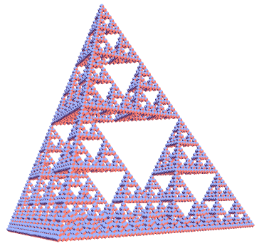

Posted in Uncategorized | 8 Comments

Cipher 30: Finale

Posted on May 21, 2013 by apgoucher

This is the final cipher of the first season on cp4space. This will be followed by a short period of cp4space aestivation, estimated to be about two or three weeks, before the next season of ciphers commences. Don’t worry; there will still be regular cp4space articles in the interim, although I cannot make any promises about their frequency.

V3,L6,T3,G6,X9,D9,L1,V6,M7,K8,E3,Z9,V5,R6,Y1,Q1,X2,E5,P8,P7,M1,
C4,R2,A4,S7,Y6,Y14,T9,E3,W8,X5,H4,W8,T8,P2,O9,T8,F5,Z4,H1,P3,
U7,X11,H1,R4,D8,E3,Z5,C2,S6,U5,O7,Y4,V4,M10,C4,M5,P10,A8,H6,L2,
I2,O12,F5,O6,X1,Y2,S5,O4,O9,P4,J8,Z2,H3,S11,V1,E9,V5,J2,V7,C1,
Z1,P10,Y3,R1,S5,I4,Y10,I6,G6,P5,B6,T10,U6,G6,E10,C1,H5,K6,Y9,
H4,Y11,R3,Z6,Q1,B7,B7,Y10,G1,W5,O1,A8,D7,O4,D6,J7,M1,S7,U1,I3,
R6,X7,F5,Y4,W9,S11,T3,S7,O12,X8,Q4,E3,Z8,W8,Y7,J2,M7,K9,T6,B10,
K7,S5,X7,E1,E9,J3,W3,K2,F3,Z3,L3,X8,V5,E4,H4,I3,R5,X5,B6,C3,H3,
Z10,Y2,M5,R6,Y15,T8,E6,U4,C6,C5,B9,S8,W4,I6,O9,L2,Z7,J3,S7,N8,
P5,T3,C3,E7,N1,O12,O10,P9,B11,X11,E2,I1,E1,I2,L6,C4,O6,X7

Posted in Ciphers | 5 Comments

Hoffman-Singleton graph

Posted on May 18, 2013 by apgoucher

I’m not sure exactly how to motivate a discussion of the Hoffman-Singleton graph, except perhaps by beginning with the following problem from the October 2011 edition of the Advanced Mentoring Scheme:

This problem seems quite innocuous at first, and one would not expect there to be particularly deep mathematics associated with it. Even more surprising is that there’s a very specific unsolved problem related to this.

You might want to attempt this AMS question; it’s not particularly difficult. We can very quickly characterise these graphs as having diameter 2 (any pair of vertices can be connected by a path of length at most 2) and girth 5 (the length of the shortest cycle is 5), as well as noticing that every pair of vertices is contained in a 5-cycle, and so on. Pretty soon, it should be obvious that the smallest such graph is the pentagon itself:

Petersen graph

One may then wonder whether there are other graphs with this property. Generally, a good idea is to try your favourite graph. If you haven’t yet reached the stage where you have a favourite graph, adopt the Petersen graph as your newly-acquired favourite graph. Here are a few drawings of your favourite graph:

The leftmost diagram is the bog-standard drawing of the Petersen graph, which is the most instantly recognisable. The second one looks completely different, but more careful analysis demonstrates their equivalence. Taken together, it becomes clear that we’re dealing with a graph of immense symmetry. We can actually think of the Petersen graph as the skeleton of a dodecahedron, but with opposite vertices identified with each other. The complete graph K6 can be obtained by applying the same process to the icosahedron.

The third diagram differs only trivially from the first (there is a continuous deformation of the plane which relates them), and shows that the Petersen graph can be drawn such that all edges are the same length.

All of these drawings contain crossings, since the graph is non-planar (indeed, it is one of the simplest graphs that is not linklessly-embeddable) by virtue of having both the K5 and K3,3 as minors. It can, however, be drawn on the surface of a torus without crossings; I’ll leave the proof as an exercise to the reader.

Anyway, the point is that the Petersen graph satisfies the conditions specified in the problem.

Hoffman-Singleton graph

We’ve shown that there exist graphs of degree 2 and 3 with these properties. The next graph has degree 7, and is known as the Hoffman-Singleton graph. Noam Elkies proves its existence and uniqueness here.

Although it is not apparent from the rendering above, this graph is also massively symmetric. Ed Pegg provides a very elegant construction of the graph, which I’ll repeat below.

Consider the 35 3-subsets of {1, 2, 3, 4, 5, 6, 7}. We’ll call these triads.
Label the vertices of a Fano plane with the numbers {1, 2, 3, 4, 5, 6, 7}. By applying even permutations to the labels, we can obtain a total of $\dfrac{2520}{168} = 15$ distinct labellings of the Fano plane. Ed refers to these as fanos.
Let the 50 vertices of the Hoffman-Singleton graph be associated with the 35 triads and 15 fanos. We connect two triads with an edge if they are disjoint; we connect a triad to a fano if the former appears as a line in the latter.

It should be evident, with a little thought, that this gives a 7-regular graph. In fact, Pegg’s construction makes it straightforward to show that the conditions of the AMS problem are satisfied:

Property (i) is obvious from the fact that it’s 7-regular.
Property (ii) can be verified by a very short case check. No two fanos are connected, so three acquaintances must either (a) all be triads, or (b) one fano and two triads. Case (a) is impossible, since we cannot find three disjoint subsets of size 3 in the 7-element set {1,2,3,4,5,6,7}. Case (b) is similarly impossible, as we can’t find two disjoint lines in the Fano plane.
Property (iii) takes slightly longer to verify. We split this into four cases, namely two fanos (c), one fano and unconnected triad (d), two triads intersecting in a single point (e) and two triads intersecting in two points (f). For case (c), note that two distinct fanos cannot share two lines (lest they are identical), so can share at most one. It’s similarly impossible for two fanos to have no common lines, so they must share precisely one. The corresponding triad, and only that triad, is connected to both fanos. For case (d), the three non-collinear points in the Fano plane can be extended to a set of four non-collinear points (an oval), the complement of which is a line disjoint from the original triad. In case (e), we can trivially embed the lines in a single labelled Fano plane. Case (f) is even easier: take the complement of the union of the two triads; this gives a third triad disjoint from the other two.

Hence, we can confirm that the Hoffman-Singleton graph actually works. Hooray!

Ed Pegg actually went further than merely constructing the graph; he designed a playable card game based on it. The case-bash above is precisely the solution to Pegg’s Puzzle E, showing that any two non-connected vertices have a unique common neighbour.

Although Pegg’s construction separates the vertices into clusters of sizes 15 (the fanos) and 35 (the triads), rest assured that the graph is actually vertex-transitive and thus all vertices are equivalent.

Beyond this?

It is a theorem, the Hoffman-Singleton theorem, that any graph satisfying those three properties must have either degree 2, 3, 7 or 57. In the first three cases, existence and uniqueness have been confirmed (with the pentagon, Petersen graph and Hoffman-Singleton graph, respectively).

As for degree 57, it is unknown whether such a graph exists. I very much hope that there is a unique such graph (since it would be another exceptional object, and exceptional objects are beautiful things), and there’s probably a really clever construction. It would have 3250 vertices and 92625 edges.

Observe that the Hoffman-Singleton graph contains lots of Petersen graphs, which in turn contain lots of pentagons. Similarly, I imagine that a degree-57 Moore graph would feature a plethora of Hoffman-Singleton graphs embedded within it.

Posted in Uncategorized | 16 Comments

Simultaneous proofs

Posted on May 15, 2013 by apgoucher

Two open problems about the distribution of the primes have been solved within about 24 hours of each other, namely the ternary Goldbach conjecture and a weakened form of the twin prime conjecture. Let’s look at these in approximate chronological order:

Ternary Goldbach conjecture

This states that every odd integer $n \geq 5$ can be expressed as the sum of three primes. Hardy and Littlewood first proved this for sufficiently large integers, conditional on the truth of the Riemann Hypothesis. Later, in 1937, Vinogradov proved the result for sufficiently large numbers without requiring the Riemann Hypothesis; this became known as Vinogradov’s theorem.

An lower bound was established, which was gradually reduced to $e^{3100}$ in 2002, still ahead of the computer searches (which have only probed up to about $10^{18}$ ). Very recently, this was further reduced to 5, as desired; see the paper by Helfgott.

We can corollary-snipe† at this point, and state that this trivially implies that every integer $n \geq 8$ can be expressed as the sum of four primes. The full version of Goldbach’s conjecture is equivalent to every integer $n \geq 6$ being expressible as the sum of three primes.

Twin primes conjecture

Twin primes are primes which differ from their closest prime neighbours by 2. For instance, {5, 7}, {59, 61} and { $65516468355 \times 2^{333333} - 1$ , $1 + 65516468355 \times 2^{333333}$ } are examples of pairs of twin primes. It has been conjectured that there are infinitely many such pairs, although no proof is known (there was a purported proof in 2004, but it was fallacious).

It has now been proved that infinitely many pairs of primes have a distance of at most 70000000. Again, this can be corollary-sniped to deduce that there exists some $N \leq 70000000$ such that infinitely many pairs of primes are separated by precisely N. No explicit values of N are known, and the original conjecture states that 2 has this property.

Conclusion and footnotes

Together, these results provide another piece of evidence for the following conjecture:

There are infinitely many pairs of exciting proofs published within 70000000 milliseconds of each other.

† Corollary-sniping is a rather impolite and dishonourable practice in which one jumps on a big theorem proved by someone else, and proves one or more corollaries using it. For instance, if someone suddenly exclaimed “Hence Fermat’s Last Theorem!” just as Andrew Wiles proved the necessary cases of the Tanayama-Shimura conjecture, that would have been an epic case of corollary-sniping (if that happened, hopefully the prize would still have been awarded to Wiles). An actual instance was when Xia’s proof that particles can be projected to infinity in finite time under Newtonian gravity was famously corollary-sniped to deduce that the n-body problem is undecidable.

Posted in Uncategorized | 17 Comments

Definition

The extension property

Induced subgraphs

Uniqueness

Damaging the graph

Tearing the graph into pieces

The Random Graph

Alternative Constructions

Proving stuff about this graph is quite easy

Why you should adopt the Rado graph as your favourite graph

“But I’ve already got a favourite graph!”

Sources

Coprimality

Probabilities

Food incompatibility triad

Curvature of space

Platycosms in two and three dimensions

Poincare dodecahedral space

Moment of inertia

Mean distance

Sierpinski tetrahedron

Petersen graph

Hoffman-Singleton graph

Beyond this?

Ternary Goldbach conjecture

Twin primes conjecture

Conclusion and footnotes

Recent Posts

Subscribe to Complex Projective 4-Space

Archives

Recent Comments