Generalising Erdős’ conjecture

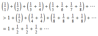
It’s a well-known fact that the harmonic series (i.e. the sum of the reciprocals of the natural numbers) diverges to infinity. There are at least two reasonably straightforward ways to prove this, the first being the Cauchy condensation test. Essentially, in this case, it involves observing the following inequality:
condensation

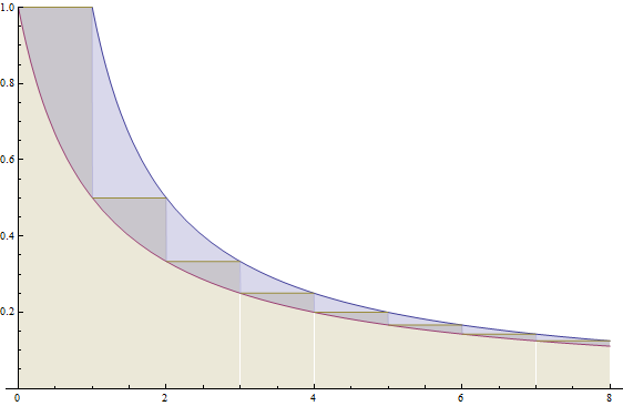
It can also be upper-bounded by a similar series, leading to the revelation that the series diverges logarithmically. Alternatively, you can obtain the result by comparing with the integral of 1/x. Specifically, the series can be expressed as the integral of a stepped function, trapped between the areas of two hyperbolae (which differ by 1).
integral-test

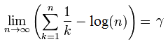
Hence, we can deduce that the following limit exists, and is bounded somewhere between 0 and 1:
mascheroni

γ is the Euler-Mascheroni constant, which is roughly 0.577.

Prime harmonic series

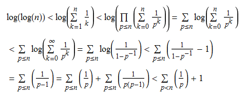
If we instead repeat this process with a subset of the natural numbers, the resulting series may converge. For instance, the sum of the reciprocals of the squares, known as ζ(2), converges to π²/6. What about the sum of the reciprocals of the primes? This turns out to diverge, albeit extremely slowly. Euler provided a heuristic argument (it lacks the rigour to be an actual proof) that it diverges at an asymptotic rate of log(log(n)). With a little work, it’s possible to rigorously prove that the sums of reciprocals of primes is bounded below by log(log(n)) − 1:
rigorous

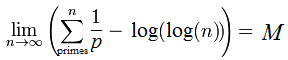
Indeed, there’s an analogy of the Euler-Mascheroni constant called the Meissel-Mertens constant:
meissel

The previous proof demonstrates that M ≥ −1. In fact, our lower bound is quite poor, as M is approximately equal to 0.2615.

Brun’s constant

The sum of the reciprocals of Mersenne primes is obviously convergent, since it can be bounded above by the series 1 + 1/2 + 1/4 + 1/8 + …, which converges to 1. It transpires that the sum of the reciprocals of twin primes also converges (the proof is much more difficult); the limit of this series is Brun’s constant. When computing the twin primes, Professor Thomas Nicely discovered a bug in the floating-point arithmetic of the Pentium processor.

Green-Tao theorem and Erdős’ conjecture

The τ theorem (named after Professors Ben Green and Terry Tao) states that there exist arbitrarily long arithmetic progressions in the prime numbers. For example, a sequence of 26 primes in arithmetic progression is {43142746595714191, 48425980631694091, 53709214667673991, 58992448703653891, 64275682739633791, 69558916775613691, 74842150811593591, 80125384847573491, 85408618883553391, 90691852919533291, 95975086955513191, 101258320991493091, 106541555027472991, 111824789063452891, 117108023099432791, 122391257135412691, 127674491171392591, 132957725207372491, 138240959243352391, 143524193279332291, 148807427315312191, 154090661351292091, 159373895387271991, 164657129423251891, 169940363459231791, 175223597495211691} (sequence A204189 in the OEIS). On the other hand, there are no infinite arithmetic progressions of primes; the proof of this is trivial.

The primes are described as a substantial set, which means that the sum of their reciprocals diverges. Erdős conjectured that the Green-Tao theorem generalises to all substantial sets, offering a prize of 3000 USD for a proof. This conjecture would generalise Szemerédi’s theorem (since all sets of positive lower density are substantial), and therefore van der Waerden’s theorem (since in any k-colouring of the integers, we can find a colour with a lower density at least 1/k). For an explanation of these theorems, together with proofs of some other generalisations, consult the third chapter (Combinatorics II) of MODA.

Generalising further?

In the same way that the Hales-Jewett theorem generalises van der Waerden’s theorem, and that the density analogue of Hales-Jewett extends Szemerédi’s theorem, it seems natural to consider this (conjectural) generalisation of Erdős’ conjecture:

  • Suppose we have a set A of natural numbers, such that the sum of the reciprocals of elements of A diverges. Write the elements of A in base n, for n ≥ 2. Then I conjecture that there exists a combinatorial line of length n.

For example, it conjectures the existence of an arithmetic progression of 10 primes, which form a combinatorial line when written in decimal. Problem 51 of Project Euler asks you to find the first partial combinatorial line of 8 primes, and provides an explicit example (56**3) with 7 primes: {56003, 56113, 56333, 56443, 56663, 56773, 56993}. If you can find a combinatorial line of 10 primes, I’ll be impressed.

One way to avoid all combinatorial lines is to take the integers whose decimal expansions do not contain any 9s. This sequence begins {1,2,3,4,5,6,7,8,10,11,12,…}. If the sum of the reciprocals of these integers diverged, then we would have a simple counter-example to my conjecture. However, it is straightforward to prove that the sum of the reciprocals of 9-less integers (the Kempner series) converges; the limit is roughly 22.92. The proof generalises in the obvious way to any combination of radix and digit.
Posted in Uncategorized | Leave a comment

Three directions

Firstly, I would like to announce that today is the Ides of March.

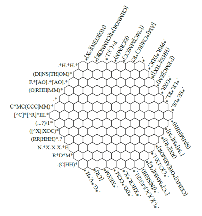
Secondly, I was alerted on two semi-recent occasions to this beast of a puzzle, namely the regular expression crossword. Like a normal crossword, you populate the empty cells of a grid with letters such that the resulting lines agree with the corresponding clues. However, as you can see below, there are a few fundamental differences:

The clues are regular expressions, which constrain the possible strings of letters. For example, the regular expression ‘[CR]*’ uses the Kleene star to enable arbitrary strings to be formed over the alphabet {C,R}. For example, CCRRC, R, CC and the empty string all fit this regular expression, whereas the string RRGCR does not. Other symbols have different properties.

Another disparity between this and conventional crosswords is the underlying lattice. Instead of the square tiling, \mathbb{Z}^2, the author has chosen to use a hexagonal tiling instead. Consequently, each cell lies on three lines, and the clues point in three directions.

This mention of ‘three directions’ provides a neat segue on to my third and final point. I feel compelled to draw your attention to an excellent music video published yesterday by the Three Directions, entitled ‘That Makes It Invertible’. Skip to 1:10 in the following video to listen to the song:

[youtube=http://www.youtube.com/watch?v=O4KCoNvRi6Y]

Posted in Uncategorized | Leave a comment

Antoine’s necklace

(Sorry about the recent dearth of cp4space postings; I’ve been rather busy in real Euclidean 3-space, \mathbb{R}^3.)

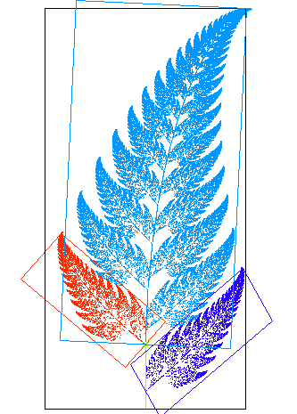
Quite a large class of self-similar geometrical objects can be expressed as iterated function systems. For instance, the Sierpinski triangle is composed of three copies of itself, each scaled by a factor of ½ and translated by a cube root of unity. More elaborate self-similar sets can be generated by applying other combinations of affine transformations, such as the Barnsley fern:

In most cases, the Hausdorff dimension is not an integer, in which case the object is referred to as a fractal. For instance, the aforementioned Sierpinski triangle has a dimension of log(3)/log(2). The Cantor ternary set, on the other hand, has a dimension of log(2)/log(3).

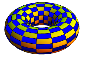
A rather paradoxical fractal is Antoine’s necklace. Firstly, you begin with a plain, bog-standard torus:

torus-grid

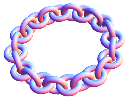
Then, place a circular chain of linked tori inside the torus, like so:

stage1

We can repeat this process inside each of these tori, and so on ad infinitum. Taking the intersection of the (nested) sets obtained at each stage, the result is homeomorphic to the Cantor set. However, the complement is not simply-connected, and therefore not homeomorphic to the complement of the usual embedding of the Cantor set in 3-space. More details are included here.

Antoine’s necklace can be used to construct another unusual object, Antoine’s horned sphere. This is obtained by taking a sphere, and extending a tentacle from its surface, which penetrates the initial torus in the construction of Antoine’s necklace. Inside the torus, the tentacle branches into more tentacles, which penetrate each of the sub-tori. This results in a tangled dendritic mess, which is homeomorphic to the 3-ball. However, quite alarmingly, the complement of the horned sphere is not homeomorphic to the complement of the 3-ball. Another such ‘exotic embedding’ of the 3-ball is Alexander’s horned sphere.

Posted in Uncategorized | Leave a comment

Cipher 20: Ulam

It’s difficult to believe that this is the twentieth cp4space cipher. Anyhow, here it is:

UTF8


Posted in Ciphers | Leave a comment

Permanent-determinant method

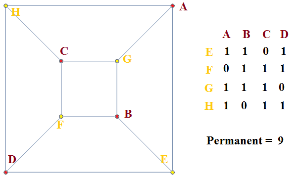
The determinant of a matrix can be regarded, most naturally, as the volume scaling factor of the corresponding linear map. However, one of the formulae for finding the determinant of a n \times n square matrix is to compute \sum_{\sigma \in S_n} sgn(\sigma) \prod_{i=1}^n A_{i,\sigma(i)}, where we sum over all permutations and take their signs into account.

But what if we omit the term sgn(\sigma)? We get a related notion, known as the permanent of a matrix. This is far less useful than the determinant, but it does have a few applications.
Perfect matchings

Suppose we have a bipartite graph, and want to compute the number of perfect matchings. In this case, we can express it as the permanent of the biadjacency matrix.

cube-permanent

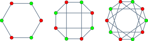
One special family of bipartite graphs are the crown graphs. A crown graph can be defined as a bipartite graph, the biadjacency matrix of which is the complement of the identity matrix. The permanent of a crown graph on 2n vertices is given by the closest integer to \dfrac{n!}{e}.

Crown graphs on 6, 8 and 10 vertices, respectively

The menage problem asks how many ways n couples (each containing one man and one woman; I apologise for the heteronormative nature of this) can be seated around a circular table of 2n seats, such that each person sits adjacent to neither his or her partner, nor anyone of the same same gender. It is not too difficult to see these arrangements correspond to Hamiltonian cycles of crown graphs. The solution sequence is given by A094047.

Domino tilings

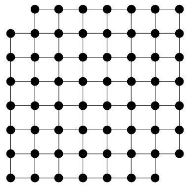
Another type of bipartite graph arises when you replace each square in a polyomino with a vertex, and join adjacent vertices with edges. For example, the bipartite graph arising from the Mutilated Chessboard Problem is shown below:

mutilated-chessboard

Since its biadjacency matrix has 32 rows but only 30 columns, it is not square and therefore does not have a well-defined permanent. Hence, there is no way to tile the mutilated chessboard with dominoes.

It transpires that in the case of tiling polyominoes with dominoes, we can define a slightly altered biadjacency matrix, by weighting vertical edges with 1 and horizontal edges with the imaginary unit i. In that case, the determinant of the new matrix is equal to the permanent of the old one, and therefore the number of domino tilings.

This may seem like a pointless modification, but it massively accelerates computation. General determinants can be computed much more efficiently than permanents, namely in polynomial time O(n^3). On the other hand, if arbitrary permanents can be calculated in polynomial time, then P = NP follows as a corollary.

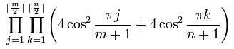
For a m \times n chessboard, the determinant of the modified biadjacency matrix was proved by Kasteleyn to have the following closed form:

kasteleyn

For m = 2, the number of tilings is the Fibonacci number F(n+1).

Spanning trees

The number of spanning trees of a particular graph can also be expressed as the determinant of a matrix, thanks to Kirchoff’s theorem. It is a remarkable fact that the number of domino tilings of a (2m - 1) \times (2n - 1) chessboard with one corner removed is precisely the number of spanning trees of a m by n grid graph, as mentioned here. Here are the 15 spanning trees of a particular grid graph, grouped into congruence classes:

congruence-classes

And here are the 15 corresponding domino tilings:

neighbours

I have joined pairs of tilings with an edge if they can be interconverted by rotating a single square of two dominoes. It has been proved that for any simply-connected polyomino, the resulting graph of domino tilings is connected. Of course, this is untrue for multiply-connected polyominoes (consider the two tilings of a 3 × 3 square with the centre removed).

In this case, the resulting graph of tilings is bipartite. This is true in general, as the number of horizontal dominoes (modulo 4) must alternate between 0 and 2 every time you move along an edge. Indeed, in the example shown above, the graph corresponds to a polyomino. This, however, is just a coincidence: with arbitrarily large polyominoes, we can get tilings with arbitrarily many neighbours.

Posted in Uncategorized | Leave a comment

Eilenberg-Mazur swindle

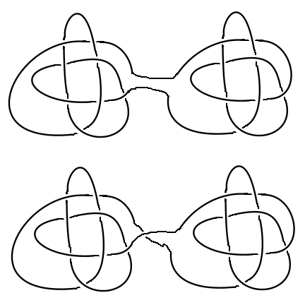
The connect sum of two knots is obtained by joining them together in the obvious way. There is, however, one small detail. If you define this naïvely, then you won’t necessarily obtain an unambiguous connect sum. For instance, consider the following:

ambiguous-sum

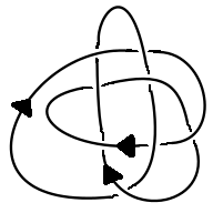
It’s difficult to show that the two above knots are non-equivalent (as usual), but it is indeed the case. The best way to avoid this problem is to consider directed knots instead of undirected knots. The knot shown below is one of the simplest ‘non-invertible knot’, i.e. one which cannot be deformed into itself such that the directions of the arrows change:

directed-knot

The first example can be viewed as the sum of two equally directed knots, whereas the second example is the sum of two oppositely directed knots. Now that we’ve imposed direction, the connect sum of knots is well-defined; I’ll leave proving it as a straightforward exercise for the reader.

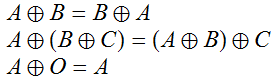
Note that connect sum is both commutative and associative, with the unknot O (simple loop) forming an identity. The set of knots under the operation of connect sum is thus an Abelian monoid.

commass

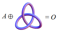
For this to be an Abelian group, we would need inverses. Unfortunately, this is not the case; for instance, there is no knot A that behaves as an ‘anti-trefoil’:

no-solutions

A simple proof of this is to note that the trefoil knot is tricolourable, whereas the unknot is not, and that the connect sum of a tricolourable knot and an arbitrary knot gives another tricolourable knot. This contradicts the above equation, so there is no anti-trefoil. Indeed, more generally, there are no two non-trivial knots A and B such that A \oplus B = O. The standard proof is the Mazur swindle:

mazur-swindle

This appears to be massively cheating. For instance, the argument could be applied to 1 and −1 to deduce that 1 = 0, which is clearly erroneous. However, it is intuitive that this reasoning works in the context of knots, since it can be realised geometrically.

Interestingly, the Abelian monoid of knots exhibits unique factorisation (Schubert’s theorem), so it suffices to categorise the ‘prime’ knots that cannot be expressed as connect sums. The knots tabulated by Rolfsen were the prime knots, the first few of which can be viewed here.

Other applications

In addition to knot theory, the principle of the Mazur swindle can be applied to other objects. For instance, we can express the free module \mathbb{Z}_6^{\infty} as the direct sum \mathbb{Z}_2 \oplus \mathbb{Z}_6^{\infty} of itself and something which isn’t a free module over \mathbb{Z}_6. Without this idea, it’s pretty difficult to find modules satisfying these properties.

Posted in Uncategorized | Leave a comment

Cipher 19: Corrupted

You were given a coded message. Unfortunately, the bottom of the page became slightly damp, rendering several of the characters illegible (these are represented by asterisks in the text below). Your challenge is to recover the password in spite of the corrupted data.

212012020212 110110022112 000011201011 120112011120 012000021102
202022011122 100201002012 000210001122 201012112202 201000102011
202022011122 012000021102 202012222021 200112120122 001200022110
221000001120 021120011112 110001221212 221000001120 010120100102
011012221201 000202100111 120000210220 012112122002 001002001212
110012122220 000202100111 022012102211 000100121012 112020210112
120200122211 111001001001 202100000112 120112011120 000202100111
120000210220 002012200102 000200212021 012010110200 120211020222
012200200120 012011222110 000020211202 200120021100 111000222121
001000110122 201110012121 100021001220 022202222101 110221011102
000010122101 120200122211 200210020011 121202120120 012011222110
000010**2101 100121122**2 02*012102*11 20020*1*2000 012220111**2
202*00**2100 202**20*1122 01***0021102 12**0*102222 201201120***
2121*00***02 20001**2*0*0 0*10*01**012 2*10*010*01* 0****0100102
1120202***** 1***11**2122 *****2122002 2021***0**12 *011*00*02**

Have fun!

Posted in Ciphers | Leave a comment

Assorted news

Some things have actually happened. A few of these are worth mentioning.

RMM 2013 results

Firstly, the results of the Romanian Master of Mathematics (RMM 2013) competition have been published. There have been two perfect scores this year (very rare for RMM), namely Ömer Cerrahoğlu (Romania) and Krachun Dmitrii (Russia). Third in line was our very own Matei Mandache, who scored an impressive 35/42, achieving a gold medal in the process. The UK team also had another gold medallist, namely Daniel Hu.

The UK team came third (beaten only by the USA and Russia), achieving two gold medals, a silver and a bronze. The two remaining contestants each had a Double Honourable Mention, which is very respectable for competitions of this difficulty.

Multicoloured ants

Tim Hutton, Ed Pegg, Georgi Gochev and Mark Jeronimus have been exploring the space of generalisation of Langton’s ant. The threshold for non-trivial examples to appear is 1 state and 2 colours; Langton’s ant lies on this boundary, as does a modification emulating binary counting.

The latest discoveries in this area include multicoloured ants that emulate Langton’s ant, but taking increasingly long amounts of time to do so. This is no longer a mystery, and can be explained by the reversibility of the original Langton’s ant. The proof of the Cohen-Kung theorem extends to show that these generalisations also settle into building a periodic highway.

For 1-state 3-colour, the 3-colour Langton Ant is beaten by a turmite that also emulates Langton’s ant, but in a very different way. Specifically, it alternates direction between forwards and backwards, and takes 18.5 million generations (as opposed to 2.67 million) before settling into a cycle of gradually increasing length. Its asymptotic growth rate is O(\sqrt(t)), where t is the elapsed time.

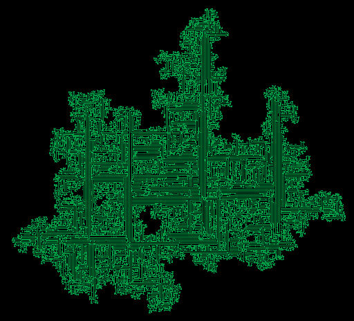
Both of these are beaten by a completely different 1-state 3-colour turmite, which takes 67 million generations to settle into a periodic highway. Here you can see the mess left behind by the turmite before escaping to the left:

1s3c-champion

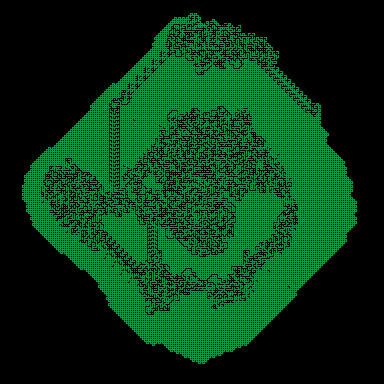
There are 9 unresolved Turmites in this space, so it is possible that there are even longer periods of time before stabilisation occurs. These have all been explored for at least 10 billion generations, and show no signs of becoming predictable. One of these exhibits binary counting behaviour:

When the amphisbaenic binary counter reaches the mess to the right, it is expected to become unpredictable again. It is unknown whether, at any time, one of these binary counters is created in a position where it would expand forever. I conjecture that this turmite does eventually become predictable. Firstly, by the Law of Excluded Middle, precisely one of the following must necessarily apply:

  1. The turmite is unbounded, and therefore the bounding rectangle must continually expand. This can only happen if the turmite touches the perimeter of the bounding rectangle infinitely often. Every time this occurs, there is a nonzero probability of producing a binary counter in such a position where it expands forever.
  2. The turmite is bounded in a N by M box, in which case it can last for at most M N 3^{M N} generations before entering a periodic cycle.
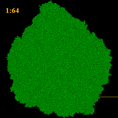
Of course, this is not guaranteed to happen, since the turmite could continually evade placing binary counters at the perimeter (similar to tossing an infinite sequence of heads on a fair coin). Alternatively, it may ultimately enter some other type of non-chaotic behaviour, such as constructing a highway (in which case it is still predictable, and therefore still satisfies my conjecture).

For 2 states and 2 colours (the subject of Ed Pegg’s turmite challenge), I mentioned how Worm Trails had been beaten twice, with the current champion lasting 240 million steps. This record has been smashed another two times. Firstly, Gochev provided one with a lifespan of 7.735 billion steps, which finishes by constructing an expanding triangular wedge:

Georgi then broke his own record rather spectacularly, giving an example with a lifespan of 3.511 trillion generations. This one eventually produces an infinite highway:

2s2c-champion

Amonst the unresolved 2-state 2-colour turmites, a few produce interesting patterns:

labyrinthine

This one produces ephemeral orthogonal and diagonal highways in its interior:

semicardinal

Posted in Uncategorized | Leave a comment

Radical Tauism

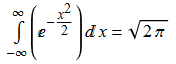
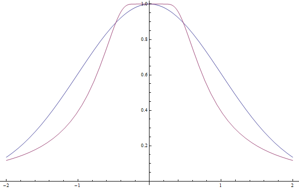
Consider the Gaussian function \dfrac{1}{\sqrt{2 \pi}} e^{-\frac{1}{2}x^2}. This gives the standard normal distribution, which has zero mean, unit variance, and points of inflection located at ±1. Note the scaling term \sqrt{2 \pi}, which is included so that the integral is 1 (necessary for a probability distribution). Specifically, we have:
normal

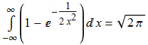
This is not so surprising, and can readily be derived from considering a two-dimensional Gaussian distribution. Much more unusual is that this related function also has an integral of √(2π) (although suitable changes of variables should relate these integrals).

antinormal

This function is much more bizarre than the normal distribution. Firstly, it is completely flat (i.e. all derivatives are zero) at its peak:

distributions

Intriguingly, it is only completely flat at a single point (unlike, say, a horizontal line segment, which is completely flat on an interval). It is quite strange for an infinitely-differentiable function to have this property, and completely impossible over the complex numbers. If we look at what happens near zero, you’ll notice some stunningly pathological behaviour:

tl-antinormal

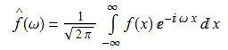
Anyway, I digress. What I actually wanted to talk about was the ubiquity of √(2π). It also occurs in the definitions of the continuous Fourier transform and its inverse:

fourier

You may have heard the amusing arguments debating whether it’s better to use π or τ = 2π as a fundamental constant. We have had a Tau Manifesto, which was soon met with criticism in the form of the Pi Manifesto. I propose a third competing faction, namely Radical Tauism (it’s funny because ‘radical’ can mean ‘(square-)root’ as well as ‘extremism’ ;P), which insists that √(2π) is better than the other two alternatives. In order to win, I suppose I’ll systematically deconstruct the arguments of the opposition parties.

Shown above is an image from the Pi Manifesto. It shows a unit circle, which has equal area to a square whose diagonal length is … erm … √(2π). Oh, yes, I forgot to mention yet another occurrence of √(2π), namely Stirling’s asymptotic formula for the factorial function.

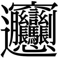
The main benefit, however, is that both pi and tau can be expressed as polynomials in √(2π), whereas the converse is false. Square roots are ugly (being multi-valued when extended to the complex plane), so it’s cleaner and more elegant to eliminate them completely by inventing a new symbol for √(2π). The question is, which symbol? We want something relatively simple, which excludes (for example) the Chinese ‘biang’ character:

I look forward to seeing your comments and criticisms.

Posted in Uncategorized | Leave a comment

Cipher 18: Enigma

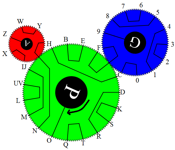
This was, as suggested by the title, inspired by the Enigma machine used to encode run-of-the-mill messages during the Second World War (more high-security messages were encoded with the Lorenz cipher). The Enigma machine was relatively easy to operate, and performed an involution (self-inverse function) to the plaintext to produce the ciphertext; this means that a single machine can be used for both encryption and decryption. If you don’t know the initial settings, however, cracking the cipher requires a huge computational effort. The cryptanalysts at Bletchley Park managed to reduce the Sisyphean search slightly by taking advantage of the fact that no letter could be enciphered as itself (unfortunately, you can’t enjoy that liberty!) and searching for expected phrases, or ‘cribs’. Even then, it took several hours of mechanised trawling to recover the initial settings of the Enigma machine for each message.

enigma

Your challenge is to determine the original position and operate the machine to decipher the following ciphertext:

HQO7CHRNUXLBIHN 1NS CPHHBT2 RPMF SBCFFM. LHF OLQFANTB XF FWNXSIIYU.

Good luck. As usual, the password is entirely in lowercase.

Posted in Ciphers | Leave a comment