Homotopy Type Theory

2017 has been an unfortunate year for Fields medallists. Maryam Mirzakhani, who won the Fields medal in 2014, passed away at the untimely age of 40. Two days ago, she was joined by Vladimir Voevodsky, 2002 Fields medallist, who was awarded the prize for introducing a homotopy theory on schemes, uniting algebraic topology and algebraic geometry.

He also defined the ‘univalence axiom’ which underpins the recent area of homotopy type theory. This is an especially elegant approach to the foundations of mathematics, with several particularly desirable properties.

Problems with set theory

The most common foundation of mathematics is first-order ZFC set theory, where the objects are sets in the von Neumann universe. It is extremely powerful and expressive: all naturally-occurring mathematics seems to be readily formalised in ZFC. It does, however, involve somewhat arbitrary and convoluted definitions of relatively simple concepts such as the reals. Let us, for instance, consider how the real numbers are encoded in set theory:

A real is encoded as a Dedekind cut (down-set) of rationals, which are themselves encoded as equivalence classes (under scalar multiplication) of ordered pairs of an integer and a non-zero natural number, where an integer is encoded as an equivalence class (under scalar addition) of ordered pairs of natural numbers, where a natural number is a hereditarily finite transitive well-ordered set, and an ordered pair (a, b) is encoded as the pair {{a, b}, {a}}.

Whilst this can be abstracted away, it does expose some awkward concepts: there is nothing to stop you from asking whether a particular real contains some other set, even though we like to be able to think of reals as atomic objects with no substructure.

Another issue is that when we use ZFC in practice, we also have to operate within first-order predicate logic. So, whilst ZFC is considered a one-sorted theory (by contrast with NBG set theory which is two-sorted, having both sets and classes), our language is two-sorted: we have both Booleans and sets, which is why we need both predicate-symbols and function-symbols.

Type theory

In type theory, we have a many-sorted world where every object must have a type. When we informally write \forall x \in \mathbb{R} . \phi(x), we are thinking type-theoretically, that ‘the proposition φ(x) holds for for all reals x’. In set theory, this is actually shorthand for \forall x . ((x \in \mathbb{R}) \implies \phi(x)), namely ‘for every object x, if x is a real then the proposition φ(x) holds’.

This idea of types should be familiar from most programming languages. In C, for instance, ‘double’ and ‘unsigned int’ are types. It is syntactically impossible to declare a variable such as x without stating its type; the same applies in type theory. Functional programming languages such as Haskell have more sophisticated type-theoretic concepts, such as allowing functions to be ‘first-class citizens’ of the theory: given types A and B, there is a type (A → B) of functions mapping objects of type A to objects of type B.

These parallels between type theory and computation are not superficial; they are part of a profound equivalence called the Curry-Howard isomorphism.

Types can themselves be objects of other types (in Python, this is familiar from the idea of a metaclass), and indeed every type belongs to some other type. Similar to the construction of the von Neumann hierarchy of sets, we have a sequence of nested universes, such that every type belongs to some universe. This principle, together with a handful of rules for building new types from old (dependent product types, dependent sum types, equality types, inductive types, etc.), is the basis for intuitionistic type theory. Voevodsky extended this with a further axiom, the univalence axiom, to obtain the richer homotopy type theory, which is sufficiently expressive to be used as a foundation for all mathematics.

Homotopy type theory

In type theory, it is convenient to think of types as sets and objects as elements. Homotopy type theory endows this with more structure, viewing types as spaces and objects as points within the space. Type equivalence is exactly the same notion as homotopy equivalence. More interestingly, given two terms a and b belonging to some type T, the equality type (a = b) is defined as the space of paths between a and b. From this, there is an inductive hierarchy of homotopy levels:

  • A type is homotopy level 0 if it is contractible.
  • A type is homotopy level n+1 if, for every pair of points a and b, the type (a = b) is homotopy level n.

They are nested, so anything belonging to one homotopy level automatically belongs to all greater homotopy levels (proof: the path spaces between two points in a contractible space are contractible, so level 1 contains level 0; the rest follows inductively). The first few homotopy levels have intuitive descriptions:

  • Homotopy level 0 consists of contractible spaces, which are all equivalent types;
  • Homotopy level 1 consists of empty and contractible spaces, called mere propositions, which can be thought of as ‘false’ and ‘true’ respectively;
  • Homotopy level 2 consists of disjoint unions of contractible spaces, which can be viewed as sets (the elements of which are identified with the connected components);
  • Homotopy level 3 consists of types with trivial homotopy in dimensions 2 and higher, which are groupoids;
  • Homotopy level 4 consists of types with trivial homotopy in dimensions 3 and higher, which are 2-groupoids, and so on.

More generally, n-groupoids correspond to types of homotopy level n+2. The ‘sets’ (types in homotopy level 2) are more akin to category-theoretic sets than set-theoretic sets; there is no notion of sets containing other sets. I find it particularly beautiful how the familiar concepts of Booleans, sets and groupoids just ‘fall out’ in the form of strata in this inductive definition.

Voevodsky’s univalence property states that for two types A and B, the type of equivalences between them is equivalent to their equality type: (A ≈ B) ≈ (A = B). Note that the equality type (A = B) is the space of paths between A and B in the ambient universe U, so this is actually a statement about the universe U. A universe with this property is described as univalent, and the univalence axiom states that all universes are univalent.

Further reading

I definitely recommend reading the HoTT book — it is a well-written exposition of a beautiful theory.

[P. S. My partner and I are attending a debate this evening with Randall Munroe of xkcd fame. Watch this (cp4)space…]

Posted in Uncategorized | 6 Comments

Wallis Workshop

We’re pleased to announce a sequel to the Ada Lovelace Hackathon. Specifically, we’re organising a workshop on Sunday 27th November 2016 to commemorate the 400th birthday of John Wallis, Cambridge mathematician and Parliament’s chief cryptographer. His developments include early analysis (infinitesimals and convergence) and the eponymous Wallis’ Product which expresses π as an infinite product expansion:

wallis

He also analysed a reciprocal structure designed by Leonardo da Vinci, resolving forces to show that it is stable without any external support. This is considered to be the first example of structural analysis, and involved solving linear equations in the 25 variables illustrated in the following diagram:

frame

He also coined the lemniscate symbol for infinity, ∞, and wrote a book on grammar. As such, broad themes of the event will include infinity, non-standard analysis, reciprocal structures, and cryptography. More suggestions are available on the website.

There will also be a baking competition, as before, and fancy dress is encouraged. If you need reminding, here is one of the entries from last year:

edible-tantrix

We’ll also endeavour to actually nominate a winner this time…

Posted in Uncategorized | 1 Comment

Is Craig Wright?

Today there has been an explosion of media interest in the claim by Craig Wright that he is the identity behind the pseudonymous creator of Bitcoin, Satoshi Nakamoto. However, his blog post is rather suspicious, as it contains various misconceptions that one would not expect from an expert in the field, let alone the originator of Bitcoin.

“A process known as combinatorics”

Several paragraphs into the post, he begins discussing technical details and making various errors:

Wright writes: The SHA256 algorithm provides for a maximum message size of 2^128 – 1 bits of information whilst returning 32 bytes or 256 bits as an output value.

No, the SHA-256 algorithm only supports inputs of length up to 2^{64}-1. Specifically, there is a preprocessing stage where extra bits are appended to the end of the input as follows:

  • Input data (n bits)
  • Padding (512 – (n+64 mod 512) bits)
  • Binary representation of n (64 bits)

This ensures that the prepared input has a length divisible by 512, which is necessary for the mixing algorithm which operates on blocks of 512 bits.

Anyway, this error is just about excusable since it pertains to the obscured internal details of an algorithm which people often use simply as a ‘black box’ for generating cryptographically secure message digests. The next sentence was much more concerning, since it suggests a serious mathematical misconception:

Wright writes: The number of possible messages that can be input into the SHA256 hash function totals (2^128 – 1)! possible input values ranging in size from 0 bits through to the maximal acceptable range that we noted above.

This does not even remotely resemble the correct number of possible inputs, which is 2^{2^{64}} - 1. The use of a factorial to count the number of binary strings should immediately trigger alarm bells in anyone with a rudimentary undergraduate-level understanding of discrete mathematics.

This is followed by the rather amusing deviation:

Wright writes: In determining the possible range of collisions that would be available on average, we have a binomial coefficient (n choose k) that determines the permutations through a process known as combinatorics [1].

The reference is to a paper by Lovasz, a great mathematician who would be either amused or offended to hear the field of combinatorics described as ‘a process‘. Moreover, binomial coefficients count subsets, rather than ‘determine permutations’, and most professional cryptanalysts would struggle to decipher the phrase ‘possible range of collisions that would be available on average’.

Nitpicking the code

In one of the images on Craig Wright’s blog post, there is a screenshot of Notepad displaying a putative shell script for verifying an ECDSA signature. With the comments removed, the code reads as follows:

filename=$1
signature=$2
publickey=$3

if [[ $# -lt 3 ]] ; then
 echo "Usage: verify <file> <signature> <public_key>"
 exit 1
fi

base64 --decode $signiture > /tmp/$filename.sig
openssl dgst --verify $publickey -signature /tmp/$filename.sig $filename
rm /tmp/$filename.sig

Note that the antepenultimate line says ‘signiture’ instead of ‘signature’, so the script doesn’t do what is claimed. In particular, it reads the signature from the environment variable ‘signiture’ rather than from the command-line argument. Hence, if you populate the environment variable with your own public-key, rather than Satoshi’s, you can cause the test to pass!

Whether this was indeed a malicious trick to convince spectators (or economists, as the case may be) or simply an innocent typo is unclear. But in the latter case, the script clearly was never tested; otherwise, the error would have been quickly detected. Either way, this seems somewhat suspicious.

“I’m Satoshi, and so’s my wife”

This is by no means the first time someone has claimed to be Satoshi. However, on this occasion there is the added caveat that two well-known Bitcoin developers, Jon Matonis and Gavin Andresen, purport that Wright is indeed right. This rules out the possibility that Wright is merely trying to seek attention, and instead suggests the following dichotomy:

  1. Matonis and Andresen genuinely believe that Satoshi is Wright.
  2. The triumvirate have ulterior motives for perpetuating a ruse.

Several explanations for (2) have been proposed. In particular, there is a rift amongst the Bitcoin developers between the ‘big-blockians’ and the ‘little-blockians’ (to parody Jonathan Swift), which I shall attempt to summarise here. Firstly, note that block size is essentially a measure of how many transactions can be handled in a 10-minute interval.

The little-blockians want the block sizes of Bitcoin to remain small, and thus for it to be a pure decentralised currency that can be used by anyone with a computer. This would maintain it as a peer-to-peer currency, but would limit its growth.

By comparison, the big-blockians believe Bitcoin should grow into a universal currency, expanding the block size to accommodate absolutely every transaction. The downside is that this is beyond the computational limits of domestic machines, thereby meaning that Bitcoin could only be regulated by banks, governments, and other large organisations: thereby moving it away from a libertarian idyll into something more akin to a regular currency.

Matonis, Andresen and Wright are all big-blockians. Having the esteemed creator Satoshi on their side would help their argument, and it is entirely plausible that there are several large organisations who would benefit from having more control over the regulation of Bitcoin.

Whether these motives are indeed the case, rather than mere speculation, will require further evidence. But as the evidence stands, I would not like to bet any money, cryptographic or otherwise, on the validity of Wright’s claim…

Posted in Uncategorized | 26 Comments

March miscellany

Several rather interesting developments have occurred this month. In inverse chronological order, they are summarised below:

E8 and Λ24 lattices actually are optimal

The lattices E8 and Λ24 are lattice packings of unit spheres in 8 and 24 dimensions, respectively. They possess many exceptional properties, including being highly symmetrical and efficient sphere packings. Indeed, it was shown that, among all lattice* packings of spheres in 8 and 24 dimensions, E8 and Λ24 have the highest density. Moreover, it was known that no packing whatsoever could be more than microscopically more efficient than either of these exceptional lattices.

*that is to say, ones where the group of translational symmetries acts transitively on the set of spheres.

Now, it has actually been proved that E8 and Λ24 have the highest density among all sphere packings, not just lattice packings. Maryna Viazovska made a breakthrough which allowed her to prove the optimality of the 8-dimensional packing; subsequently, she led a group of collaborators who refined this approach to apply to the 24-dimensional Leech lattice.

More on this story here.

AlphaGo defeats Lee Sedol in a 4-1 victory

A team of researchers at Google DeepMind developed a program to play the board game Go at the professional level. It was pitted against a 9-dan professional Go player (that is to say, one of the very best Go players in the world), Lee Sedol, winning four of the five matches. Lee Sedol was able to obtain a single victory, his fourth game, by observing that AlphaGo was less strong when faced with unexpected moves (despite having made several of its own, described by spectators as ‘creative’!).

The algorithm ran on a distributed network of 1202 CPUs and 176 GPUs. It uses a combination of brute-force tree searching (like conventional chess algorithms), Monte Carlo simulations (where many plausible futures are simulated and evaluated) and pattern recognition (using convolutional neural networks). These convolutional neural networks are much larger and deeper than the one I implemented on the Analytical Engine, with 192 feature-maps in the first convolutional layer. In particular, AlphaGo used:

  • A value network to evaluate how favourable a position appears to be;
  • A supervised policy network to learn how a human would play;
  • A reinforcement policy network to decide how it should play;
  • A fast rollout policy network which is a simpler, cruder, and faster counterpart of the above (used for the Monte Carlo rollouts).

The supervised policy network was trained on a huge database of human matches, learning to recognise spatial patterns with its convolutional networks. After quickly exhausting the database, it had no option but to play lots of instances of itself via reinforcement learning, using competition and natural selection to evolve itself. In doing so, AlphaGo had effectively played more matches than any human had ever seen, growing increasingly powerful over a period of several months (from when it played the 2-dan European Go champion Fan Hui).

A much more detailed description of the algorithm is in the Nature paper.

Unexpected pattern discovered in Conway’s Game of Life

It transpires that, despite 46 years of interest and hundreds of thousands of CPU-hours of Monte Carlo searching, there was a piece of low-hanging fruit in an area no-one had thought to explore. This was the copperhead, a spaceship with the unusually slow speed of c/10:

copperhead

Alexey Nigin wrote an excellent article describing its discovery. In the next few days after the article’s publication, there were additional breakthroughs: Simon Ekström discovered that the spaceship could be extended to produce a profusion of sparks:

tagalong

This extension is capable of perturbing passing objects, such as reflecting gliders. A convoy of these creatures can consequently catalyse more complex interactions, such as duplicating and recirculating gliders to yield an unterminating output; the following example was constructed by Matthias Merzenich:

sokwe-rake

As you can see, there is a steady stream of NE-directed gliders escaping to the right.

Posted in Uncategorized | 4 Comments

Presidential endorsement paradox

Posted in Uncategorized | Leave a comment

Deep Learning with the Analytical Engine

In December we held a hackathon to celebrate the 200th birthday of Ada Lovelace. In the last post, the results of the baking competition were mentioned along with our efforts to program the Analytical Engine emulator. Although I briefly alluded to a project I undertook last month which built upon these ideas, the implementation was only completed a few hours before I had to present it in a talk. As such, the actual results are hitherto undocumented, except in the deepest recesses of a GitLab repository.

The project was to implement a machine-learning algorithm within the confines of the Analytical Engine (which amounts to about 20 kilobytes of memory and a very minimalistic instruction set). If you have 35 minutes to spare, here is my talk introducing the project. My apologies for the hesitant beginning; the talk was unscripted:

It transpired that, at the time of the talk, there were a couple of mistakes in the implementation; I was later able to detect and remove these bugs by writing additional Analytical Engine code to facilitate debugging. After making these modifications, the machine-learning code learned how to recognise handwritten digits surprisingly well.

As mentioned in the talk, a simple neural network would occupy too much memory, so I implemented a deep convolutional network instead (with extra optimisations such as using the cross-entropy cost function and L2 regularisation in the final fully-connected layer). Specifically, there are 5 feature-maps in the first convolutional layer, and 10 in the second convolutional layer:

convnet-complete

Code generation was performed by a combination of a Bash script (for overall orchestration) and several Python scripts (for tasks such as generating code for each layer, implementing a call-stack to enable subroutines, and including the image data in the program). The generated code comprises 412663 lines, each one corresponding to a punched card for the actual Analytical Engine. Even if the punched cards were each just 2mm thick, the program would be as tall as the Burj Khalifa in Dubai!

The following progress report shows a dot for an incorrect guess and an asterisk for a correct guess; it is evident that the code is rapidly learning:

first-epoch

You can see during the first training epoch that its performance increases from 10% (which is expected since an untrained network equates to random guessing, and there are 10 distinct digits {0, 1, 2, 3, 4, 5, 6, 7, 8, 9}) to 79% from training on 5000 images. This was followed by a testing phase, in which a different set of 1000 images were presented to the network without the labels; unlike in the training phase, the network isn’t given the labels for the testing images so it cannot learn from the test and subsequently ‘cheat’. The testing performance was 79.1%, broadly in line with its performance on the training data towards the end of the epoch as one would expect.

We then repeat this process of training on 5000 images and evaluation on 1000 images. The performance improved again, from 79.1% to 84.9%. After the third epoch, it had increased to 86.8%, and by the end of the ninth epoch it had exceeded 93%. At that point I accidentally switched off my remote server, so the results end there. If you set the program running on your computer, it should overtake this point after about 24 hours.

[Edit: I subsequently tried it with 20000 training images and 10000 evaluation images, and the performance is considerably better:

  1. 89.69%
  2. 93.52%
  3. 94.95%
  4. 95.53%
  5. 95.86%
  6. 96.31%

and is continuing to improve.]

Theoretically the architecture should eventually reach 98.5% accuracy if trained on 50000 images (confirmed by implementing the same algorithm in C++, which runs about 1000 times more quickly); I urge you to try it yourself. Complete source code is available on the Deep Learning with the Analytical Engine repository together with additional information and links to various resources.

Posted in Uncategorized | 9 Comments

Lovelace hackathon: results

In the previous post, I mentioned the hackathon we were organising to celebrate the 200th birthday of Ada Lovelace. The event was a huge success, and it is safe to say that all attendees had a most enjoyable, creative and productive time. For posterity, here is a recount of the various aspects of the hackathon.

The baking competition

Many of the attendees produced delicious treats in advance of the hackathon. These were designed to sustain us throughout the latter half of the event (i.e. after the café upstairs closed at 16:00). Everyone else constituted a committee of ‘impartial judges’ who would decide amongst themselves the winning entry. But before I announce the results, here are the entries:

Edible Tantrix tiles (Simon Rawles, Deepa Shah, Adam P. Goucher):

edible-tantrix

We only had three colours of icing and an insufficient amount of gingerbread to constitute a standard-issue Tantrix set (cf. the decidedly inedible tiles surrounding the plate). Also, I was responsible for cutting the hexagons and was in something of a rush due to having to catch a bus back to central Cambridge in time for a feast.

Hackathon title (Jade-Amanda Laporte, Jardin-Alice Laporte)

laporte-title

Delicious, pertinent, and with a stylised ‘200’ resembling the digits embossed on the wheels of the Analytical Engine.

Miscellaneous shapes of variable genus (origin unknown)

variable-genus

Definitely the tastiest three-holed torus I’ve encountered.

Hyperbolic tessellation (Tim Hutton, Neela Hutton)

hyperbolic-tiling

Somewhere between the Poincare and Beltrami-Klein models.

The results

The impartial judges were far too terrified to vote! Due to fear of offending the other entries, they didn’t reach any conclusion! As such, no entry was declared the winner, much to the disappointment of the contestants.

Programming the emulator

We succeeded in implementing an absolute-value function and (later) an activation function for a neural network, verifying its correctness using the Analytical Engine Emulator.

kali-aes

After a while, we managed to get an actual plot of the activation function using the Curve Plotting Apparatus (which Babbage proposed as part of his design for the Analytical Engine). This research eventually culminated in a project to realise a machine learning algorithm on the Analytical Engine (cp4space post coming soon!).

Posted in Uncategorized | 1 Comment

Ada Lovelace Day: 10th December 2015

After several months of planning, I would like to announce that there will indeed be an event in Cambridge to celebrate the 200th birthday of Ada Lovelace (10th December 2015):

http://www.cambridgelovelace.org/

The organising committee is composed entirely of volunteers, so the event is completely free to attend: just turn up on the day! Details, including the date, time and location, are on the official website in addition to the Facebook event page.

We hope to see you there!

Posted in Uncategorized | Leave a comment

Superflip composed with fourspot

Somehow, it slipped past my radar that Tomas Rokicki and Morley Davidson have established the maximum number of quarter-turns necessary to solve a Rubik’s cube (the more widely-popularised figure of 20 was for the half-turn metric). That is to say, any of the six faces can be rotated by 90° clockwise or anticlockwise in a single move.

We can consider the Cayley graph, which is 12-regular (since at each position, there are 12 possible moves one can make) and bipartite; this is most easily seen by noting that a quarter-turn induces an odd permutation (a 4-cycle) on the eight vertices of the cube. Then the maximum number of moves necessary is, by definition, the diameter of the Cayley graph.

Anyway, the diameter of the graph is 26, and surprisingly there are very few positions which take 26 moves to solve (compared with billions of distance-20 positions in the half-turn metric). Indeed, it is conjectured that there are only three such positions, or one up to isomorphism: the so-called superflip composed with fourspot. It is worth explaining this terminology.

The superflip is the unique non-identity element in the centre of the Rubik’s cube group where every cell remains in its original position, but with all 12 edge cells reversed. Since it commutes with every element, the order of composing it with fourspot is not important.

The fourspot is a common pattern where four of the face cells undergo a derangement, and all other cells remain unchanged. Somehow, the fourspot has acquired something of a cult following, and even boasts its own music video:

In other news, the Erdos discrepancy problem was recently solved by Terry Tao. There is a natural way to turn this into a two-player game. Specifically, Alice and Bob take turns colouring positive integers (cobalt blue for Alice and moss green for Bob), and the game terminates when there exists a progression {n, 2n, 3n, …, kn} (for some positive integers k and n) such that the difference between the number of cobalt blue elements and moss green elements in that progression exceeds d (a predetermined constant that determines the difficulty of winning).

Also, there’s a petition for LEGO to produce a Lovelace and Babbage themed set. You’re strongly encouraged to support the petition; more information is available over at the Aperiodical. This is currently in the limelight due to Ada Lovelace’s impending 200th birthday (this December); watch this cp4space for more details of Lovelace-themed events in the coming months…

Posted in Uncategorized | 1 Comment

Coverings, convolutions and Corbynatorics

Amidst Saturday’s turmoil, the following problem came into consideration:

There are plans to build a nuclear power station on an initially empty 12-by-12 chessboard. Doing so would require an empty 4-by-3 or 3-by-4 rectangular region of squares. To foil this plan, Jeremy decides to erect coal mines on squares of the chessboard (with each mine occupying a single square) to ensure there is no sufficiently large empty rectangle. What is the minimum number of coal mines necessary for Jeremy to prevent the construction of the nuclear power station?

With little effort, one can obtain a lower bound of 12 by partitioning the chessboard into twelve disjoint rectangles, noting that each one must contain at least one mine:

lower-bound

Similarly, we can establish an upper bound of 16 by placing a mine at (x, y) if and only if x and y are both divisible by 3. Can this bound be improved? In particular, note that it is never wise to place a coal mine near the edge of the board, since we can move it inwards without reducing its effectiveness for blocking potential nuclear power plants. Without loss of generality, we will therefore only consider arrangements where the mines are in the 8-by-8 ‘reasonable region’ in the middle of the board:

reasonable-region

One reasonable approach is to place mines on the boundary of this region, and then concentrate on the centre of the board. This reduces the upper bound from 16 to 12, and is therefore optimal:

construction-12

What about a larger board? In particular, what is the lowest density of mines that can be placed on the infinite plane to leave no 4-by-3 or 3-by-4 rectangle unoccupied? Again we have a lower bound of 1/12 and an upper bound of 1/9. The upper bound can actually be reduced to 1/10 by using the following lattice:

det10lattice

It appears that it would be difficult, if not impossible, to improve upon this. Observe that if an empty 3-by-3 box occurs in any valid configuration, then there must be a coal mine in each of the four surrounding 1-by-3 boxes. Moreover, the lattice shown above achieves this bound, and has no 3-by-3 boxes containing more than one mine.

But how would one prove optimality? Given an arrangement of mines, we define a scoring function over \mathbb{Z}^2 
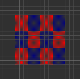
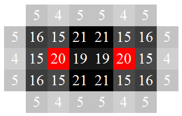
by means of a convolution. Specifically, each mine contributes a score to its own square and those surrounding it as follows:

mine-convolution

That is to say, each mine contributes a score of 20 to its own cell, 15 to the four edge-adjacent cells, 16 to the four other vertex-adjacent cells, 4 to the four cells at a distance of 2 in a horizontal or vertical direction, and 5 to each of the eight cells a knight’s move away from the mine.

Then the score associated with a given square is simply the sum of the contributions from nearby mines.

This may appear to be a seemingly arbitrary scoring function, but it was chosen to exhibit the following properties:

  • The score associated with the density-1/10 lattice is uniform across all cells (and equal to 20);
  • For any valid configuration (one with no 3-by-4 or 4-by-3 empty rectangle), every cell gets a reasonably high score (in this case, the minimum possible is 15).

Since the total score contributed by each mine is 200, we can determine the density by dividing the average score by 200. Hence, proving that the density-1/10 lattice is optimal is equivalent to the following statement:

The average score in any valid configuration must be at least 20.

It transpires that this is true, and can be obtained by locally perturbing the scoring function (without violating conservation of total score) so that no cell has a score below 20. This is a finite check, and sufficiently small that it can be performed without the assistance of a computer.

Suppose we have a cell with a score strictly less than 20. It is easy enough to show that one of the following two possibilities must arise:

  • Case I: The score is 19, and the cell is positioned between two mines like so:

two-mines

  • Case II: The cell belongs to precisely one empty 3-by-3 region, which is surrounded by four mines.

We deal with all instances of Case I before Case II, by incrementing each ’19’ and decrementing the two cells which are edge-adjacent to the ’19’ and vertex-adjacent to the neighbouring mine. This actually decreases the overall score, so (if we can show that the average score is still at least 20) any configuration with an example of Case I is suboptimal.

Case II is more complicated to address than Case I, because each of the four mines surrounding the 3-by-3 region can be in any of three possible positions. Moreover, empty 3-by-3 regions can potentially overlap slightly. Nevertheless, if we consider only the portion of the 3-by-3 region which belongs to no other 3-by-3 regions, the average score is still at least 20, with equality if and only if the mines are arranged to resemble a portion of the density-1/10 lattice. This is true even after we perform any reductions associated with Case I.

Convincing yourself is a matter of testing each of the possible sub-cases for Case II (there are at most 81, and this quickly reduces when you take symmetry into account).

What have convolutions ever done for us?

In addition to solving this rather niche problem in Corbynatorial geometry, convolutions have a wealth of other applications.

  • Even if we restrict ourselves to considering convolutions of an arbitrary function on a square grid with a small finitely-supported kernel, this is useful for image-processing. Common edge-detection algorithms use this concept, right up to the sophisticated convolutional neural networks underlying Google’s image recognition software. These are explained very clearly in various places.
  • A continuous analogue is taking a convolution of measurable functions over \mathbb{R}^n 
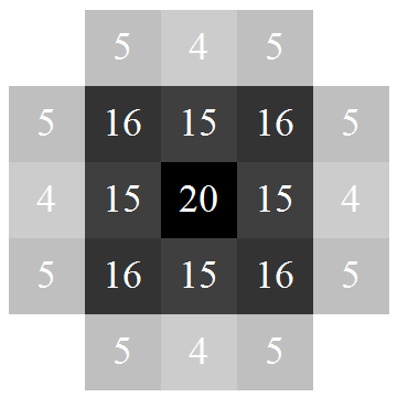
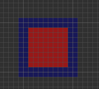
or the torus obtained by quotienting by a lattice. Gaussian kernels are often used.
  • More generally, one can convolve continuous functions over an arbitrary compact group. In the cases where the group is Abelian, this can be computed quickly by means of a Fourier transform (although this is typically overkill when the kernel has small finite support).
Posted in Uncategorized | 2 Comments