Complex Projective 4-Space

Some of my favourite books were written by Douglas Adams. (Indeed, my forename was actually named after his surname, rather than my Biblical namesake or the Greek word for ‘indestructible’.) Although I personally prefer the Dirk Gently books, I have to say that one of my favourite quotes is from the Hitchhiker’s Guide to the Galaxy:

It was on display in the bottom of a locked filing cabinet stuck in a disused lavatory with a sign on the door saying ‘Beware of the Leopard’

This reminds me of how a particularly insightful 20-year-old e-mail from John Conway is ‘on display’ in the password-protected archives of an obscure mailing list. Rather interestingly, the e-mail originated from speculation as to whether gliders are possible on a Penrose tiling. It took almost two decades for this question to be answered (in the affirmative), after the question was raised independently by Andrew Trevorrow and Tim Hutton.

[youtube=http://www.youtube.com/watch?v=6xVLpP25DRQ]

Conway recounts how he had considered automata on Penrose tilings, but subsequently rejected them in favour of simpler Turing-complete models of computation. One of his ideas was for a universal system that changes its topology, rather like how neurones in the human brain can connect, separate and reproduce with miraculous results. Some very early work in this area was by Alan Turing himself, described in The Emperor’s New Mind and summarised here.

A ‘full adder’, a basic arithmetical circuit, composed entirely of NAND gates

Basically, Turing reasoned that since NAND gates are capable of arbitrary finite computations, such as basic arithmetic, then in a very large, random mass of interconnected NAND gates, it might be possible for intelligence to arise. He referred to these as A-type machines.

However, in the human brain, connections are continually made and broken. He added extra provision (a ‘connection modifier’), resulting in the concept of a B-type machine. Of course, the connection modifiers themselves can be built from NAND gates, so there is no need to physically make and break connections.

Conway’s idea was more abstract than this, involving a (multi?)graph that evolves according to specific, local rules. I think that the closest realisation of this was Hiroki Sayama’s Generative Network Automata, although I am unaware whether any further developments have been made in this area.

Even simpler systems

At the moment, the candidates for ‘simplest universal system’ include Rule 110, a one-dimensional cellular automaton proved universal by Matthew Cook, Alex Smith’s 2-symbol 3-state Turing machine, and the SK combinator calculus. There’s an even simpler system (a Post-tag system), but it is not known whether or not it’s capable of universal computation.

Of course, the universality of Alex Smith’s Turing machine was discovered 14 years after Conway’s e-mail, which continues:

    This reminds me of my Jugendtraum, which is to find a still simpler kind of universal system that just plays one game with an infinite deck of numbered cards, and can be programmed just by suitably stacking the cards.  The rules are simple – eg., if you see a card numbered n, move n places right and reverse the order of the cards you move over (and maybe negate them).  [negative n are allowed]

It’s important that whatever the rule is, there’s only one of it – the “machine” that plays this game doesn’t have a varying “state”.  But somehow this simple rule can be programmed to compute any computable function of m,n,… just by starting it at a,b,c,…,m,n,…  for a suitable finite string a,b,c,…  (the program).

I got some rather messy rules, but still think that there should be a simple one.  The dream is that “the nice rule” is more or less unique, and astonishingly simple, and leads to a complete reformulation of the theory of computable functions.

Whilst none of the results of this search satisfied him, a few beautiful fruits grew out of this ambition. One of these was Conway’s Game of Life, which grew extraordinarily popular during the 1970s thanks to a column by Martin Gardner in the Scientific American magazine.

FRACTRAN

The other, which I’m going to mention here, was a truly remarkable ‘programming language’ called FRACTRAN. The current state of the automaton is an integer, N, and the transition rules are a list of fractions. For example, one of Conway’s programs begins with N = 2 and has the following fourteen transition rules:

On each step, multiply N by the first fraction that results in an integer. In this case, we multiply it by to give N = 15. Then we multiply it by , giving N = 825, since none of the others gives an integer. Now we can multiply it by to give N = 725. The first few integers obtained are as follows:

2, 15, 825, 725, 1925, 2275, 425, 390, 330, 290, 770, 910, 170,
156, 132, 116, 308, 364, 68, 4, 30, 225, 12375, 10875, 28875,
25375, 67375, 79625, 14875, 13650, 2550, 2340, 1980, 1740, 4620,
4060, 10780, 12740, 2380, 2184, 408, 152, 92, 380, 230, 950, 575,
2375, 9625, 11375, 2125, 1950, 1650, 1450, 3850, 4550, 850, 780,
660, 580, 1540, 1820, 340, 312, 264, 232, 616, 728, 136, 8, 60,
...

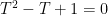
If we run it for longer and look at the powers of two that appear, we get {2, 4, 8, 32, 128, 2048, …}. Ignoring the initial 2, these are precisely  for prime p. In other words, this sequence of fractions computes prime numbers! This may seem miraculous, and indeed it is impressive, but the underlying mathematics is actually quite banal.

Note that we’re working with just the multiplicative structure of the integers, and don’t care about the additive structure. In this format, it is most convenient to consider only the prime factorisation of the fractions. Shown below are the exponents in the prime factorisations of the first few fractions.

• 17/91 –> (0, 0, 0, -1, 0, -1, 1, 0, 0, 0)
• 78/85 –> (0, 1, -1, 0, 0, 1, -1, 0, 0, 0)
• 19/51 –> (0, -1, 0, 0, 0, 0, -1, 1, 0, 0)

Essentially, FRACTRAN uses each of the exponents in the prime factorisation of N as registers to store nonnegative integers, and the fractions increment and decrement the registers according to whether or not they are empty. In this way, it behaves as a counter machine, the same model of computation I used to prove the Turing-completeness of three-dimensional chess.

He wrote two other programs, a universal computer with just 21 fractions and a 38-fraction machine for generating the decimal expansion of pi. The latter (avaliable here, although apparently slightly erroneous) is massively inefficient, using Wallis’ product. Conway also provided an initial value of N to instruct the universal 21-fraction machine to emulate the 38-fraction machine…

There are several mathematical heuristics (it’s difficult to call them proofs), which are non-rigorous in the best of cases and sometimes seemingly insane. For example, Euler’s ‘proof’ that the sum of the reciprocals of the primes diverges at an asymptotic rate of manipulates divergent series as though they were convergent, and does other dubious steps such as taking the logarithm of infinity.

He proceeded to conclude the rate of divergence of the series. It transpires that whilst the proof was non-rigorous, one can easily repair it, in this case by replacing the infinite summations with partial sums and taking the limit. It’s very messy, though, but still possible (I recall doing this for an earlier cp4space post).

Seven trees in one

Whilst the Euler proof cheats slightly, it may appear to the untrained eye to be completely legitimate. We’ll now take a look at a more extreme example, which appears more like a mathematical joke than a proof, but again reaches a correct conclusion. Later, a rigorous general proof was published, stating ‘whenever this silly approach is employed, and certain constraints are obeyed, the result of this process is a true statement’.

The subject is Andreas Blass’ Seven Trees in One, which I would probably rank among my favourite mathematical papers. Essentially, the heuristic argument runs like this:

• Consider binary trees (with ordered leaves), and let each leaf be coloured with one of k colours. Here are a few examples of trees:

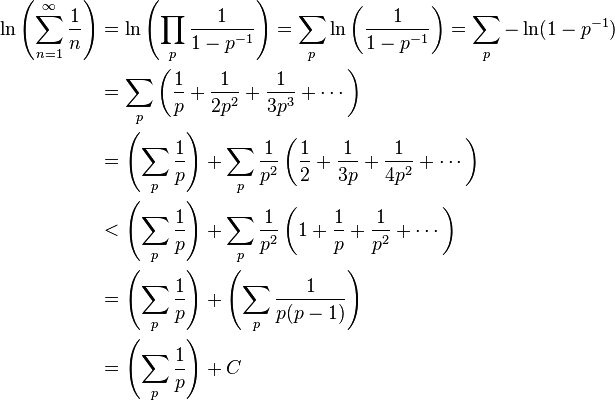
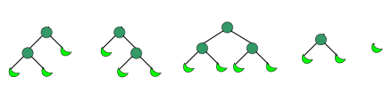
• There are trees with n leaves, thus if we colour the leaves. Hence, the total number of trees with coloured leaves is given by the series , where the coefficients are Catalan numbers. This generating function has the closed form .
• Evaluating this at gives us the number of unlabelled trees, 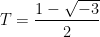. The astute observer will notice that this is a sixth root of unity, so .
• Hence, there is an elegant bijection between trees and 7-tuples of trees.

Blass then provides such an elegant bijection in the paper. Here is a diagrammatic representation of the bijection, where the letters a, b, c, … represent arbitrary trees (including the ’empty tree’ consisting of a single leaf). To use this diagram, apply the first rule that applies to your 7-tuple.

Why does this work?

It is obvious that there were many non-sequiturs in the above derivation. Nevertheless, Blass provided a rigorous justification of this argument.

• A tree is either a leaf or an ordered pair of trees (the children of the root node). Hence, it makes sense to write T = 1 + T² (where T is the set of trees, multiplication corresponds to Cartesian product, ‘+’ gives the disjoint union of two sets, and ‘=’ means ‘there exists a natural bijection’).
• Now, if we were in a ring, we could rearrange to give and multiply by to give the desired equality, . However, this argument would also give clearly erroneous statements such as . The reason this fails is that we’re not in a ring, but a semiring (ring without negatives).
• Nevertheless, in a semiring we can still apply the formula T = 1 + T² to ultimately derive the desired statement. Dan Piponi created a video, where a penny can bifurcate into two pennies in adjacent locations (corresponding to bijecting from the set of trees to the disjoint union of the singleton set and the set of ordered pairs of trees). The reverse process can also happen (since bijections are, by their very nature, invertible):

[youtube=http://www.youtube.com/watch?v=vtCV7JOnlhc]

If we replace each of these steps with the elementary bijection, the whole thing gives the bijection from trees to 7-tuples of trees.

In Einstein summation convention, repeated indices are summed over. For example, . If a Kronecker delta has two different suffices, we can ‘contract’ them as follows: , whereas .

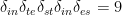Vishal Patil considered contracting English words in this manner. For example, ‘intestines’ gives us the expression . In general, suppose we have a word W of 2n letters (n pairs of distinct letters in some permutation), and wish to evaluate it in summation convention. Then the product of the deltas evaluates to , where c is the number of cycles in the n-vertex (multi-)graph produced by joining two vertices with an edge if the corresponding indices share a delta. The graph corresponding to ‘intestines’ is shown below:

English words consisting entirely of repeated letters

I wanted to find other examples (other than ‘intestines’) of words in the English language which feature each letter precisely twice. To do so, I downloaded the official Scrabble dictionary SOWPODS (verifying that it was comprehensive by checking that it contains the word ‘boustrophedonic’) and wrote the following simple Mathematica program:

As you can see, there are a couple of 12-letter words in there, namely ‘trisectrices’ and ‘happenchance’. Conveniently, 12 is a multiple of 3, so we can evaluate the product of Levi-Civita symbols with these subscripts:

Here I’ve used the fact that the Levi-Civita symbol is invariant under cyclic permutations, and then simplified the expression using epsilon-delta contractions. We can also evaluate ‘trisectrices’:

You can have a go yourself at evaluating expressions corresponding to other English words.

Sum of all words

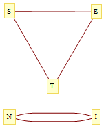
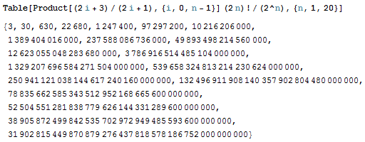
Suppose we evaluate each of the permutations of aabbcc…dd (with 2n letters) using Kronecker deltas (as we did with intestines) and wish to sum them together. For , we just have one word with a value of 3. For , we have six words, two of which have a value of 9 and four of which have a value of 3, so the sum is 30. We can continue this sequence.

If we choose a random word on n letters, the probability generating function for the number of cycles is given below:

Setting s = 3 gives us the expected value of a random word. Multiplying this by the number of words will thus give us the total:

This sequence is already in the OEIS as A007019, but there is no mention of it being equal to the ‘sum of all words’ in Einstein summation convention.

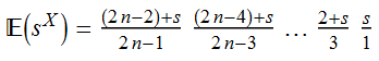
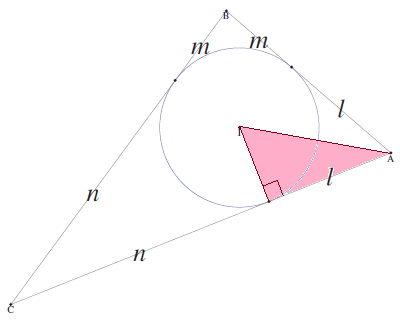
Sam Cappleman-Lynes noticed the seemingly remarkable fact that at least one of the interior angles of a triangle being equal to π/3 is equivalent to the linear relation between the semiperimeter, circumradius and inradius. He provided a clever synthetic solution, and I demonstrated that a mindless algebraic bash (starting from the cosine rule) will also give the same result, where a quartic factor drops out of a sextic to leave a quadratic, which is miraculously the square of a linear term.

This problem made its way onto a sheet of ‘background problems’ at the 2013 Easter Trinity camp. Gabriel Gendler recognised it as being very similar to a theorem he had already seen, namely that a triangle satisfies if and only if it is right-angled. At this point, I conjectured that for every angle , the existence of at least one angle of θ in the triangle is equivalent to some homogeneous linear equation in (R, r, s).

It transpires that proving even this more general statement is not too difficult, and far more straightforward than any of the solutions presented to the background problem at the Trinity camp. The techniques here are described in MODA, but I’ll assume that you haven’t necessarily read it (or, if you have, remembered it) and include everything here.

The original solution was so hideously complicated as a result of using the cosine rule. Instead, we’ll use a simpler tangent rule, which facilitates a much shorter proof. If you concentrate on the rose-tinted right-angled triangle in this diagram, you should observe that .

So, the condition that at least one of the angles of the triangle is θ is the following cyclic product, which evaluates to zero if and only if at least one of the factors is zero:

We then expand this as a cubic polynomial in . Each of the resulting elementary symmetric polynomials in (l,m,n) can be converted into polynomials in (R,r,s) using the ‘symmetric polynomial conversion toolkit’, resulting in the following:

After dividing throughout by a factor of r², we obtain a homogeneous linear relationship in (R,r,s) as desired:

Relation to cubic curves

Homogeneous linear equations in three variables correspond to planes through the origin in three-dimensional Euclidean space, . Here, the planes corresponding to angles of 30°, 60° and 90° mutually intersect on a line, representing a set of similar triangles:

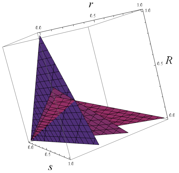
However, homogeneity enables us to reduce them to lines on the real projective plane , where points on the projective plane represent different similarity classes of triangles.

As θ varies, the line on the projective plane moves in a weird way. Using projective duality, however, we can make more sense of this. We now have a point for each value of θ (thus the locus, rather than the envelope, is a curve), and a line passing through that point corresponds to a similarity class of triangles with at least one angle of θ. Isosceles triangles are lines tangent to the curve (therefore doubly intersecting the same point, corresponding to two copies of that angle), and the equilateral triangle is the line tangent to the point of inflection. Our 30°-60°-90° triangle is the line suggested by these three collinear points:

This ‘dual curve’ is actually a cubic, which endows it with a beautiful Abelian group operation by virtue of Cayley-Bacharach (c.f. elliptic curve calculator). In this case, it embodies the fact that the interior angles of a triangle sum to π. I have always said that practically all of Euclidean geometry can be deduced from Cayley-Bacharach, but I didn’t imagine that the geometry of the triangle was so intimately related to elliptic curves.

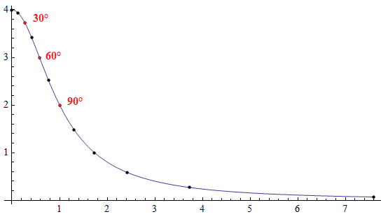
The card game Set is played rather regularly at gatherings such as the MathsJam events held nationwide on a monthly basis. The original game involves trying to identify sets of three cards which form lines in the affine hyperspace . Here is an example of such a set:

Each card can be represented by a vector . Each coordinate represents one of the four attributes (quantity, shape, colour and shading, in that order), and is interpreted modulo 3. The three cards shown above are , and .

This coordinate system is somewhat unsatisfying, due to the presence of an ‘origin’. To circumvent this, it is necessary to prepend another coordinate, , to produce projective coordinates. The leftmost card in the diagram above is now 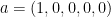. We can now identify the necessary and sufficient condition that three cards form a ‘set’ (henceforth referred to as a line, since it’s more accurate):

• Line: Three linearly dependent vectors, no two of which are identical.

Equivalently, we want three vectors, , such that some linear combination of them (with coefficients of ±1) equals the zero vector. By considering the fixed coordinate, it is evident that the number of ‘positive’ terms in the linear combination differs from the number of ‘negative’ terms by a multiple of three. In this case, the only admissible equation for a line is this:

• Line: Three vectors a, b, c, such that .

These definitions are more mathematically interesting than the seemingly arbitrary (albeit equivalent) rule of ‘either all the same or all different, for each attribute’. Also, the first one lends itself particularly well to a generalisation (named after Edward Kirkby, who proposed this major modification to the rules of the game):

• Kirkby: Four coplanar points, no three of which are collinear.

An example of a Kirkby

By the same argument, the only possible structure for a Kirkby is a set of four vectors satisfying . This was the standard definition of a Kirkby for quite some time, so it was only recently that Gabriel Gendler realised that lines and Kirkbies were special cases of a (potentially infinite) sequence. His own surname became associated with the next term, defined thusly:

• Gendler: Five cohyperplanar points, no four of which are coplanar.

The desired structure is . If this equation is obeyed and there are no lines, then we can deduce that there are also no Kirkbies and thus we have an actual Gendler.

Restricting ourself to four-dimensional space, there is only one more term. I’m not precisely sure of the exact etymology of this, but I believe that the following name and definition became associated:

• Carlotti: Six points in general linear position.

Since we have six cards, it is necessarily true that any one can be expressed as a linear combination of the other five. In particular, there are two admissible structures for a Carlotti, namely and .

Any affine transformation in this space can be expressed uniquely as a matrix with 20 variable entries (the top row is fixed). Consequently, the group of invertible affine transformations is transitive on sets of five points in general linear position. A corollary is that any two lines are equivalent, any two Kirkbies are equivalent and so are any two Gendlers.

We can generalise to more dimensions. At a Cambridge MathsJam, the clumsy dining abilities of one of the attendees led to the idea that three packs of Set cards, each one of which has been smeared with a different flavour of preserve (strawberry, blackcurrant and apricot, for an explicit example). In this case, Carlotties are no longer in general linear position, and a different type of structure arises.

This is breaking news, by the way; hence, the article is somewhat rushed. (If you haven’t heard of Conway’s Game of Life, there is a summary on Wikipedia.)

As of a few minutes ago, Mike Playle discovered a π/2 stable reflector with a recovery time of 43 generations, which is an order of magnitude faster than its competitors. Here it is in the form of the first period-43 oscillator; it can be trivially modified to yield any period ≥ 43 (including 53, which hadn’t been attained until now).

Due to the small size of 19 × 23 pixels, he wins a prize of $100 from Dave Greene, which had remained unclaimed for twelve years! Similarly, the fast recovery time of 43 generations earns an additional $100 from Matthias Merzenich. It appears that Ed Pegg’s prize puzzle page needs updating to reflect (no pun intended!) this discovery.

Coincidentally, the beta of Golly 2.5 has also just been released.

Slightly older news

Also recent, but not quite as recent, was Josh Ball’s discovery of a tiny c/7 spaceship. There are now nine orthogonal spaceship velocities, summarised in this infographic I prepared earlier (note the Ford circles):

Dave Greene, Hartmut Holzwart and I are currently involved in the process of engineering a 31c/240 spaceship, so that might be appearing reasonably soon. It is likely to be rather large, though.

Twelve years ago, Kontsevich and Zagier published an enlightening exploration of a set of real (or, more generally, complex) numbers known as periods. Firstly, let’s have a look at which sets are subsets of which other sets:

The integers  are a proper subset of the rationals , which are in turn a subset of the algebraic numbers (roots of polynomials with integer coefficients, such as  and i/92 amongst other things). The algebraic numbers are a dense subset of the complex plane. Dan Christensen plotted the roots of polynomials of low degree with small coefficients:

Despite being dense in the complex plane, roots of reasonably small polynomials are quite far apart; large holes occur around 0, 1, i and other points, devoid of close algebraic approximations. The real line is also very densely populated, since (for instance) every polynomial of odd degree has at least one real algebraic root.

The field of algebraic numbers is actually quite tame, and we can easily verify whether two algebraic numbers are equal (use Euclid’s algorithm to extract the greatest common divisor of the corresponding polynomials and observe whether or not they share that root). By contrast, this does not apply in the set of computable complex numbers; there is no algorithm for proving that two Turing machines generate the same computable number. We don’t even know whether the Euler-Mascheroni constant γ is rational!

To summarise, algebraic numbers are well understood, whereas computable numbers are deeply mysterious and enigmatic. The algebraic numbers are rather restrictive, excluding important mathematical constants such as π and e. It would be nice to have a larger set of well-understood numbers; this was the motivation for Kontsevich and Zagier’s study.

What is a period?

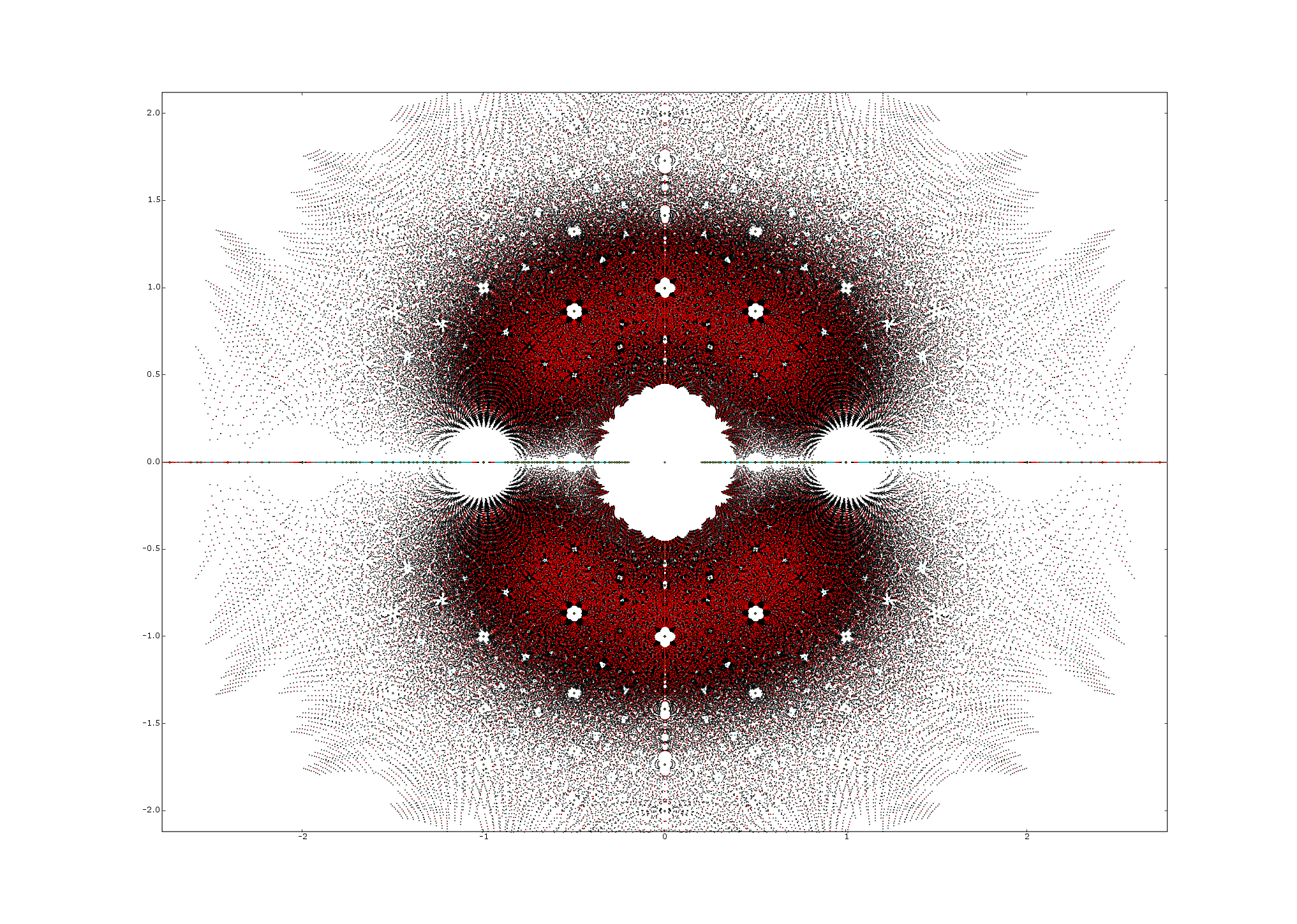
A number is a period if it can be expressed as an integral of a rational function over a region of  determined by polynomial inequalities with rational coefficients (together with Boolean operators). For example, π is a period, since it can be expressed as the integral of 1 over the domain . Periods are closed under multiplication (take the Cartesian product) and addition (express the integrals as volumes of regions determined by algebraic inequalities, and take the disjoint union of the resulting regions). Hence, the periods form a ring .

Examples of periods include:

• π (area of a circle);
• Logarithms of algebraic numbers (integrate 1/x from 1 to α);
• Zeta function at integer arguments (including ζ(3), Apery’s constant);
• Elliptic integrals;
• Γ(p/q)^q;
• The lemniscate arc length, S.

The authors of the paper also consider the extended period ring, where 1/π (which is conjecturally not a period) is adjoined to the ring. These rings are equal if and only if 1/π is a period. It is not even known that the periods do not form a field, although this is widely believed to be the case.

All periods are computable (do numerical integration in your favourite computer algebra software running on a Turing machine), so basic uncomputable numbers such as Chaitin’s constant Ω aren’t periods. There is also a just-do-it construction for a computable non-period: start with an enumeration of the periods, and choose your favourite closed interval [a,b]. For each period, select a smaller closed interval (in a computable way) that avoids that period. The intersection of these intervals is a single real number, which is computable but not a period. A more explicit example of a non-period has since been found, analogous to how Liouville constructed a transcendental number.

Identities between periods

In the paper, Zagier and Kontsevich conjectured that two integrals correspond to the same period if and only if they can be related by the following operations:

1. Linearity of integrals;
2. Changes of variables (such as affine transformations);
3. The Fundamental Theorem of Arithmetic and generalisations to higher dimensions.

For example, we can formulate ζ(2) = π²/6 in two completely different ways:

• The integral of 1/(y − x y) over the region 0 < x < y < 1.
• The integral of 1/6 over the four-dimensional region x² + y² < 1; w² + z² < 1.

It transpires that these integrals can indeed be interconverted by use of these three basic operations. If the conjecture is true, we could algorithmically decide whether any two periods are the same: alternate between numerically calculating them (to see whether they are not equal) and trying sequences of basic operations (to see whether they are equal).