Cipher 10: 2013

Assuming that this has been timed correctly, it should appear after the first minute of the first day of the new year. To celebrate this, today’s cipher is simply a matrix of 2013 binary digits. I’ll include this in both a pictorial and textual format.

1011111111111111111111111111111111111111111111111111111111101
0101111111111111111111111111111111111111111111111111111111010
1011100000001100101001010000100011111000110011001101010011101
1110000000101101101011010000000100000011100001010100000000111
1110010110100001111101111001110100000101011101100110101100111
1110010110001100011000110111011000000101100100110010101100111
1110010110001100010110101001110000000110011000110010101100111
1110011111011110110011100001110000000111101000110111011000111
1110000000000000000000000000000000000000011101010001110100111
1101110011101000101001000001011010101100111111111111111010011
1100000011010001101101010001000000000000001100010101010101011
1100111001100000001111110000101010101011011110001000100010011
1111101110110001100010100001101010101011111111011101110111111
1110111010110001100010100001101010101011111111011101110111111
1110111010110011110111110001101010101010011110001000100010011
1110000001010100000000000000000000000001001100010101010101011
1100011101010110111101011000111000001101100100000101111011011
1101011000001001000101000110001011010100000010110110101100011
1100100011001100001111110000111001110011010111001101011001111
1111111011000101001011000110001100011001010101111001011101011
1111111011000101001010110110001011010111010101111001011101011
1111111111100101001110011111001011010101101101001101011001111
1110000000001001000000000000101100011000111000110100000100011
1101010011000111101100101011100100010100110010101011000010011
1101010010100001001101011001101011010110101010001011111000111
1100100110000011101010111101111101100101011011000100010111011
1111111011010010100111100100010110110011110001001111011001011
1111111010100010100111100100010110110011110011011111100110011
1100100010100010100010111101111100110001011101110100111010011
1101010011010001001101010000000001010110101000011011000111111
1001010011011101011101000010000011001110100000011011001100001
0101111111111111111111111111111111111111111111111111111111010
1011111111111111111111111111111111111111111111111111111111101

By golly, that looks difficult!

As usual, there is a secret area of cp4space, which you’ll be able to access if and only if you’ve solved the cipher. The password is entirely in lowercase.

Posted in Ciphers | Leave a comment

Recapping 2012

Now that the year is drawing to a close, there are a few things worth discussing. Firstly, cp4space has a total of over 20000 views and a new seasonal banner (see above)!

Mathematica 9

The Treefoil has been mentioned on mathpuzzle.com. I updated the page to reflect the optimised 9-by-9-by-9 Treefoil, rendered below using Wolfram Mathematica 8:

treefoil-optimised

It turns out that a composite function I defined (to draw a three-dimensional binary array as an arrangement of cubes) has now been added to the native instruction set of the newly-launched Mathematica 9. Here’s a screenshot from the Wolfram Blog showcasing this new command:

One of the many new features of Wolfram Mathematica 9

Cipher Tuesday

I’m pleased with how well the weekly cipher challenges are going. The next one goes online at 00:01 GMT on the 1st January 2013, so if you’re in another time zone you can celebrate the new year without sacrificing your chances of being the first to solve it.

Things became interesting in November, when Vishal Patil and Sam Cappleman-Lynes decided to compete to solve as many ciphers as possible. Vishal solved the fifth cipher first, but Sam has since overtaken him and is now in a comfortable first position. Due to Vishal’s Python breaking (I hope he meant the programming language!), Joseph Myers and Maria Holdcroft have been able to overtake.

Of course, the situation may change after the next cipher is published. The leaderboard reflects the current status of which ciphers have been solved by whom.

Turing and turing

As you know, 2012 was the centenary of the birth of Alan Turing. There has been lots of well-deserved hype surrounding this, including a petition to place Alan Turing on the new £10 note. There was partial success in this direction, in that a special Bletchley Park edition of the board game Monopoly included money featuring the father of computer science*.

Donald Knuth (responsible for LaTeX and Knuth’s up-arrow notation, amongst other things) has suggested the verb ‘to ture‘ as a back-formation of Turing. He defined it as ‘to use the Internet’, thereby filling a semantic hole in the English language. Note that in the Aperiodical article, they have included his middle initial: ‘Donald A. Knuth’. It’s pleasing to see that I’m not the only middle-initialism-ist**.

The idea of back-formating† a surname to create a verb is not completely original. Whilst in a pub in Oundle, James D. Cranch contemplated the meanings of the verbs ‘to gouch’ and ‘to gendle’. The latter has since been accepted to refer to a technique of questionable legality in the game of Ultimate Frisbee, whereas my name does not yet have any semantic value. If you have any proposals, please suggest them in the ‘comments’ section of this post.

Footnotes for this section

* You could argue that either Charles Babbage or John von Neumann could warrant this title. For the former, I disagree on the grounds that whilst Babbage did design the first programmable computer (again, this can be debated; the Jacquard loom accepted a sequence of instructions, but it wasn’t used for computation so I’m not including it), he didn’t formulate the concept of universality. As for von Neumann, his research post-dated Turing’s.

** I’m not responsible for this clumsy hyphenated mess, by the way, but I choose to accept it for the sake of historical consistency.

† Yes, that was deliberately ironic and self-referential†.

Museum of Mathematics

The Museum of Mathematics opened in New York City. It is of a similar style to the earlier Eames Mathematica exhibit (bizarrely, neither related to Suzanna E. Eames nor to the aforementioned Wolfram Mathematica), featuring visual and interactive demonstrations. It’s best demonstrated by the following video:

[youtube=http://www.youtube.com/watch?v=jK7xPo1YXzY]

The museum (affectionately known as MoMath) was designed by the geometer George W. Hart. You may know him from his amazing work in polyhedra (both research and art), or via his daughter Vi. He uses 3D printing technology (which is becoming increasingly popular) to produce some elegant polyhedral sculptures. I intend to do use similar methods to build copies of a polyhedral {sculpture, knot-theoretic link, puzzle, proof that A5 is isomorphic to I, promotional item, …} to offer as prizes for the EGMO. I’ll elaborate on this very shortly…

Posted in Uncategorized | Leave a comment

Busy beavers

This is the third out of a series of four articles on increasingly fast-growing functions. The first article described the Ackermann function (corresponding to ω) and the Goodstein function (corresponding to ε_0). The second article went into much more detail about a specific function, namely Friedman’s TREE() function, giving an improved lower bound for TREE(3) in terms of the related tree() function. All of the functions we’ve encountered are computable, i.e. it’s theoretically possible for a computer to evaluate the function.

We use an idealised form of computer, the Turing machine. This has an unbounded tape of cells (one cell for each integer), each of which contains a symbol (typically an integer between 0 and m − 1, where m is the number of distinct symbols). Initially, all cells are initialised with the blank symbol 0. The machine starts on one of the cells of the tape, and has an initial ‘state’ (an integer between 1 and n).

  • Read the symbol σ in the cell where the machine is situated;
  • As a function of σ and the current state s of the machine, write a particular symbol in the cell, move either left or right, select a new state, and optionally halt.

Some machines halt, and others don’t. The busy beaver function S(n,m) is defined to be the longest halting time of any of the n-state m-symbol Turing machines that do halt. S(n,2) grows really fast, and will eventually overtake TREE(n) (probably before n = 1000). It grows faster than any computable function, so must therefore be uncomputable (indeed, it’s equivalent to the Halting Problem).

Here are some particular values and lower bounds for the 2-symbol busy beaver function:

Turmites

Although these machines are no more powerful than ordinary Turing machines, people have investigated generalisations where the tape is Z^2 rather than Z. The most familiar example is Langton’s Ant, which has an incredibly simple definition but takes about 10000 steps before settling into a periodic behaviour. The tape after 11528 steps is shown below, where the periodic ‘highway’ is clearly visible:

langton-ant

Someone decided to name these multi-dimensional Turing machines ‘turmites’, as a portmanteau of ‘Turing’ and ‘termites’. They behave in interesting ways, such as the one below. This generates a spiral of squares, the side lengths of which grow like the Fibonacci sequence:

golden-spiral

One can devise a busy beaver function for these two-dimensional Turing machines; Tim Hutton has collected some preliminary results. Georgi Gochev discovered a few 5-state 2-colour two-dimensional Turing machines with long lifespans.

Paterson’s worms

A particular finite class of Turing machines on the hexagonal lattice are rather interesting in the diversity of patterns they can create. For instance, one of these ‘Paterson’s worms’ produces an expanding Star of David (image courtesy of Benjamin Chaffin):

worm-1544152

Another one, ‘worm 1042020’, takes an enormous 57493855205939 steps before eventually halting to produce the following intricate configuration (zoomed out by four orders of magnitude):

worm-1042020

It was simulated to completion by Tom Rokicki, who designed a Hashlife-based algorithm to vastly accelerate the computation. There is currently only one worm with an unknown fate, known simply as ‘worm 1042015’. It doesn’t halt within 10^21 timesteps, and is extremely chaotic as far as it has been simulated.

Equivalent busy beaver functions

In the fast-growing hierarchy introduced in the first post, the busy beaver function would correspond to the Church-Kleene ordinal ω1CK. Rather than using Turing machines, there are many other definitions which achieve this growth rate. Here are two examples:

  • The diameter of the largest unit disc which can be covered by a set of n Wang tiles incapable of tiling the whole plane;
  • The longest time taken for a tree of n elementary combinators to eventually β-reduce to its minimal form.

The second of these alternatives will be explained in more detail in the fourth article, where I’ll generalise it to define a function far beyond the busy beaver function. I haven’t yet determined the ordinal corresponding to this function, but a lower bound is ω1CK^2. (I suspect this lower bound is very poor.)

Posted in Fast-growing functions | Leave a comment

The inadequacy of SCLT

As I mentioned a few posts ago, I included the Diophantine equation x^4 + y^6 = z^10 on the Advanced Mentoring Scheme. I’m not going to spoil it here, although I have since been informed that I had previously included it as an exercise in MODA.

Let’s consider the weaker equation, a^2 + b^3 = c^5. It’s quite easy to solve it using the good old Sam Cappleman-Lynes technique (henceforth abbreviated to SCLT), beginning with a solution to d^2 + e^3 = f. The simplest solution to this is 1 + 1 = 2, which we’ll then multiply throughout by 2^24 to give an integer solution to the original equation.

  • 4096^2 + 256^3 = 32^5

Note that 4096, 256 and 32 are not coprime by any stretch of the imagination. Can we find a coprime solution to a^2 + b^3 = c^5 in the positive integers? I stumbled across an interesting discussion which demonstrated a geometrical construction for the Diophantine equation a^4 + b^3 = c^2. I’ll explain and apply it to the more flamboyant case of our equation, which is intimately connected to the geometry of the icosahedron.

The geometry of the icosahedron

The twelve vertices of the icosahedron can be partitioned into three concentric congruent golden rectangles, the perimeters of which form Borromean rings:

Golden rectangles

The side lengths of the rectangles are in the ratio 1 : φ, where φ = (1 + sqrt(5))/2 is the golden ratio. We’ll use this later. Firstly, note that the icosahedron can be inscribed in a sphere. We then identify this (the Riemann sphere) with the extended complex plane (like C, but with a point at infinity) by stereographic projection. This is another recurring theme in MODA.

stereographic

We can see instantly that the lowest vertex is at 0, and the one diametrically opposite is at ∞. There’s still a complex degree of freedom left, which we’ll choose carefully to give the neatest expressions for the remaining vertices. Let’s choose a pair of antipodal vertices to lie on the real line, and take a cross-section of the sphere:

cross-section

Let the diameter BD be 1. Then, we can deduce that the points on the horizontal line are positioned at ψ and φ, the two roots of z^2 − z − 1 = 0. By symmetry, we get that the twelve vertices are the roots of the projective equation xy(y^5 − φ^5 x^5)(y^5 − ψ^5 x^5) = 0, which expands out to f(x, y) = x y^11 − 11 x^6 y^6 − x^11 y = 0; the coefficient ’11’ comes from being the fifth Lucas number. Hence, plotting the roots of z^11 − 11 z^6 − z = 0 in Wolfram Alpha will give you the vertices of a stereographically projected icosahedron.

wolframalpha

Hessians and Jacobians

Following the instructions in the e-mail, we compute the Hessian h and Jacobian j of f and h. These are the determinants of matrices of partial derivatives. After scaling to make the coefficients smaller, we get:

  • h = x^20 − 228 x^15 y^5 + 494 x^10 y^10 + 228 x^5 y^15 + y^20
  • j = x^30 + 522 x^25 y^5 − 10005 x^20 y^10 − 10005 x^10 y^20 −
    522 x^5 y^25 + y^30

Amazingly, we have the identity h^3 − 1728 f^5 = j^2, which holds for all complex values of (x,y). (That’s not the only place where 1728 appears as a scaling factor!) We can recover a solution to the original equation by applying a subsitution:

  • a = j
  • b = −h
  • c = 1728^(1/5) f

Now, these aren’t integer polynomials in x and y, so we rescale by letting x = 16^(1/5) s and y = 9^(1/5) t. If we substitute s = t = 1 we get a solution in the integers, but a couple of the values are negative. If we try s = 2 and t = 1 instead, the results are positive. This leads to a valid positive integer solution where a,b,c are coprime:

  • 127602747389962225^2 + 196120763999^3 = 7506024^5

As an exercise, you might want to do the same with the octahedron to get a solution to a^2 + b^3 = c^4 with coprime terms. Enjoy!

Beal’s conjecture

This is almost (but not quite) a counter-example to Beal’s conjecture. This claims that for a solution to a^l + b^m + c^n with l,m,n > 2, the integers a,b,c share a common factor. It is obvious that this (if true) implies Fermat’s last theorem, since from a solution to a^n + b^n = c^n we could divide throughout by gcd(a,b,c)^n to obtain a coprime solution. Not that this is of much interest, anyway, since we already know that Fermat’s last theorem is true.

Unfortunately, the geometric method cannot be applied to generate a solution with all exponents greater than 2, and SCLT just gives massive common factors. This is one of the many Annoying Aspects of Mathematics. Another example is that the only pairs of positive integers (m,n) for which 1² + 2² + 3² + … + m² = n² holds are (1, 1) and (24, 70), and it’s impossible to dissect a 70 by 70 square into squares of side lengths 1, 2, …, 24. Indeed, it’s an open problem with a $100 prize as to whether there exists a rectangle which can be dissected into squares of side lengths 1, 2, …, m. By comparison, Beal’s conjecture holds a $100000 prize.

Posted in Uncategorized | 3 Comments

Cipher 9: Christmas cryptography

Being simultaneously Christmas Day and Cipher Tuesday, I have a lot of material to get through.

Isaacs

Firstly, happy 370th birthday to Sir Isaac Newton, who succeeded Isaac Barrow as the Lucasian Professor of Mathematics (both from Trinity, yay!). This gives a nice segue into the topic of Isaacs, one of whom is obsessed with putting counters on chessboards in problems on the British Mathematical Olympiad:

Isaac has a large supply of counters, and places one in each of the squares of a 8 by 8 chessboard. Each counter is either red, white or blue. A particular pattern of coloured counters is called an arrangement. Determine whether there are more arrangements which contain an even number of red counters or more arrangements which contain an odd number of red counters.

This was from BMO1 2010/11. There are 1716841910146256242328924544641 arrangements with an even number of red counters, whereas there are merely 1716841910146256242328924544640 with an odd number of red counters. A random ‘even’ configuration is shown below:

isaac-random

If you solve it with Burnside’s lemma to treat rotations as equivalent, the difference is much more pronounced (429210477536564523837299872481 compared with 429210477536564060582231136160).

A couple of years later, for BMO 2012/13, Isaac resurfaced again:

Isaac places some counters onto the squares of an 8 by 8 chessboard so that there is at most one counter in each of the 64 squares. Determine, with justification, the maximum number that he can place without having five or more counters in the same row, or in the same column, or on either of the two long diagonals.

Some of the solutions people submitted were rather interesting. One person got a result of 39 instead of 32 by allowing counters to straddle boundaries between squares. Because this is a slightly less trivial problem than the intended question, I’ll include a solution to this misinterpretation:

isaac-misinterpreted

Solution with 4.875 counters in each row and column, and 1.75 on each long diagonal

Another submission involved an expletive (‘we rearrange the chessboard and this is s**t’). I don’t know whether he was describing the problem as trivial, or whether he was trying to describe the permutation (1 4) in S4 (which does rearrange ‘this’ to ‘s**t’).

Joseph Myers enumerated the number of possible solutions to the problem, arriving at 43346734009 (fourth term of A220350, which Joseph added to the OEIS recently). For the misinterpretation, there are obviously 2^aleph-null solutions.

Christmas crackers

Secondly, here are a few mathematically-themed potential Christmas cracker jokes. I apologise that these are nowhere near as good as Vishal’s puns, but it’s a well-known fact that Christmas cracker jokes are meant to be terrible. For instance, there are a few oldies based on fruit and vegetables:

crackers1

Fred Lunnon and I were responsible for the penultimate and final jokes, respectively. Slightly less family-friendly is this dreadful one of mine:

crackers2

Even more racy is the Story of Polly Nomial, which for some peculiar reason is on the website of Susan Stepney (one of the people to investigate cellular automata on Penrose tilings). Stranger still is the fact that we haven’t yet co-authored a paper together. I don’t know who wrote the story, but I was informed of its existence by James Gazet.

Anyway, you’re probably eagerly awaiting this:

The cipher

I think that my last bunch of cryptographical conundrums was slightly too difficult (possibly frustratingly so). So, this is not particularly hard by comparison:

SILPNSHGLTNUPSMLAFDCBDMWPNYDLWPNGNMSLTVUNMUHTDXXDAPHXQ
DUSDCDLUPSNAWNMWTMHGSNANUHPLPNUSIDVFILSLPNQNPLTPVQPSLS
VSLDAHDVPIDVUWCLAWLSVAVPVNUUHWLCCLTVUSUNTRDCPGNTLAFDMG
VATSVNSLDANUUDBPCDMNWWLSLDANUTDXGULTNSLDAPINGGHTIMLPSX
NPHDVBLUUBNASXHGNPPBDMWBILTILPPNSVMANULNBLSIADTNGLSNUP

Viszontlátásra

Some of the cp4space readership are going to Hungary the day after tomorrow. If you fall into this category, then I hope you thoroughly enjoy it. Interestingly, it was in precisely the same hotel (the Öreg-tó Club) that the idea of Complex Projective 4-Space was first popularised. Hence, I suppose you could consider it to be the birthplace of this blog.

Merry Christmas!

Posted in Ciphers | Leave a comment

The world still exists

It transpires that the world didn’t actually end yesterday. At the very least, Descartes’ famous deduction ‘cogito ergo sum’ seems to imply that. To summarise, the Mayan calendar has finished its 13th long count cycle; equivalently, 13×20×20×18×20 days have passed since the beginning of the aforementioned calendar. Suffice it to say, it was rather anticlimatic, with nothing particularly interesting happening.

Depicted below is a tiling of a triangular arrangement of hexagons of side length s = 9 with trihexes. An interesting problem, solved by John Conway, asks which side lengths can actually be tiled with trihexes.

T9

Obviously, it can be done in the cases s = 2 and s = 9, and it’s vacuously true for s = 0. Can we do it for other sizes? Yes, we can attain 11 and 12 by augmenting the previous tiling:

11and12

You can also add multiples of 12 rows by the following scheme, thereby attaining any side lengths congruent to {0, 2, 9, 11} mod 12.

plus12

It’s trivially obvious that you can’t tile a triangle with side length congruent to {1, 4, 7, 10} mod 12, since the number of hexagons is not divisible by 3. This leaves the cases of {3, 5, 6, 8} mod 12, which are impossible for more subtle reasons. We can convert this problem into one on a square grid by applying an affine transformation:

squaregrid

Can we tile this with L-trominos in two orientations? If we consider the perimeter of the region to be a group word (where a = up, b = left, a’ = down, b’ = right), then the two types of tromino are equivalent to the relations bbaa = abab and aabb = baba. Under these relations, the perimeter (which reduces to bbbaaab’a’b’a’b’a’) is not equivalent to the identity, so we can’t tile the entire area with trominos. This can be proved by constructing a group where the relations bbaa = abab and aabb = baba hold, but where bbbaaa ≠ ababab. Some example groups are mentioned here.

Posted in Uncategorized | Leave a comment

Dissecting the disc

At the tenth Gathering for Gardner, Colin Wright proposed the following problem. It’s quite well known, and I believe it has been published elsewhere before:

‘Dissect a [unit] disk into congruent parts at least one of which avoids the center by a positive distance’.

Bill Gosper posted this to the math-fun mailing list, where it attracted quite a lot of attention. Several people subsequently solved it, including Neil (Bickford?) and Jessica (Kleber?). It is by no means obvious that such a solution should exist, although the pieces must satisfy certain properties, such as having both convex and concave circular arcs of equal curvature to the unit disc. Invariably the first solution that people encounter is this one:

After a little additional thought, other solutions present themselves, such as the one below:

Both of these solutions use curvilinear triangles as the basic unit. It’s possible to fully characterise and enumerate all possible solutions involving curvilinear triangles. The proof is a messy geometrical case-bash, which involves showing that:

  • The only possible combinations of edges are {convex, convex, concave} and {convex, flat, concave}.
  • The length of each curved edge is strictly less than π.
  • The interior angles sum to strictly greater than π.
  • For the solution with three curved edges, two of the edges must be of equal length (isosceles curvilinear triangle). From there, one can deduce that this length is equal to 1 (consider both areas and the difference between the convex and concave arc lengths). The smallest concave edge must be a divisor of the length of the largest concave edge, whence we get that there are 6n pieces.
  • For the solution with two curved edges and one straight edge, the angle opposite the convex edge is a right angle. It transpires that no solution exists other than the symmetrical dissection into 12 pieces.

Using Burnside’s lemma (MODA, chapter 1) and a boring combinatorial case-bash, these solutions can be exhaustively enumerated. Treating congruent solutions as being the same, the number of solutions for 6n pieces is given by {0, 31, 57, 99, 158, …} (A193362) (the exceptional case where the pieces have a flat edge is included in the number 31).

The thirty non-exceptional dissections into 12 pieces

The thirty non-exceptional dissections into 12 pieces


Posted in Uncategorized | Leave a comment

TREE(3) and impartial games

This article was originally supposed to be about TREE(3) and the busy beaver function. However, I realised the potential of turning TREE(3) into a two-player finite game, which is surprisingly fun and means that I’ve ended up leaving uncomputable functions until a later post.

Last time, we explored a fast-growing hierarchy of functions. We considered the Goodstein sequence (or rather, the essentially equivalent problem C8′) to produce a function approximately equal to f_(ε_0), where ε_0 is a rather large countable ordinal. Applying this construction recursively would correspond to ordinals such as ε_0 + ω, which are not much larger than ε_0. So, if we want faster functions, we need more powerful ideas.

Friedman’s TREE(3)

Usually, we expect fast-growing functions to have a relatively smooth, steady start. For instance, the Ackermann function begins {3, 4, 8, 65536, 2↑↑(2↑↑65536), …}, and the first four terms are quite small. By contrast, the function TREE begins with TREE(1) = 1, TREE(2) = 3 and TREE(3) is so vastly, incredibly large that it greatly exceeds anything you can express in a reasonable amount of space with iteration, recursion and everything else mentioned in the previous post, including C8′ and the Goodstein function.

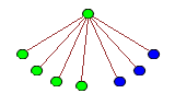
So, what exactly is TREE? The definition is quite simple, once we’ve defined a few terms along the way. We consider rooted k-labelled trees, which are connected acyclic graphs where one vertex is identified as the ‘root’, and each vertex can have one of k colours. An example is shown below:

3-labelled tree

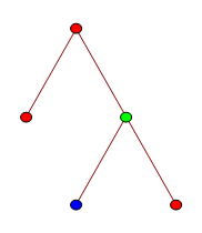
There is a binary operator, inf (not related to the infimum of a set), which returns the latest common ancestor of two vertices. Consider the tree above. If the blue vertex is called x and the green vertex is called y, then x inf y = y. Similarly, the inf of the two non-root red vertices is the root vertex.

We say that a tree S is homeomorphically embeddable into a tree T if there is an injection φ from the vertices of S to the vertices of T such that:

  • φ(z) and z have the same colour, for all z in S;
  • φ(x inf y) = φ(x) inf φ(y), for all x,y in S.

Equivalently, this means that T is a topological minor of S (where we direct the edges to respect the root vertex). The first tree is homeomorphically embeddable into this one:

tree2

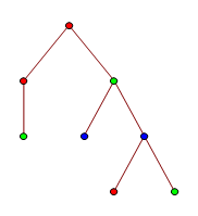
Proof: Delete the two green leaves, then contract the double-edge containing a blue vertex.

If we have an infinite sequence of k-labelled trees {T_1, T_2, T_3, …}, where each T_n has at most n vertices, then Kruskal’s tree theorem states that some T_i can be homeomorphically embedded into a later T_j. Hence, by compactness, there exists some value TREE(k), which is the length of the longest possible sequence of k-labelled trees {T_1, T_2, …, T_TREE(k)} such that |T_n| ≤ n (for all n) and no earlier tree can be homeomorphically embedded into a later tree.

Longest 2-labelled sequence

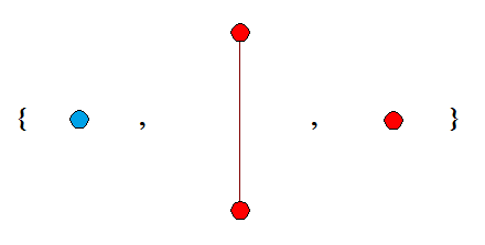
The sequence above is the longest such sequence of 2-labelled trees, so TREE(2) = 3. For any sequence, the first tree must be a single isolated vertex, and that colour is not allowed to occur in any later tree. The proof follows trivially. Now consider 3-labelled trees. We can have an extremely long sequence, such as one which starts like this:

first20

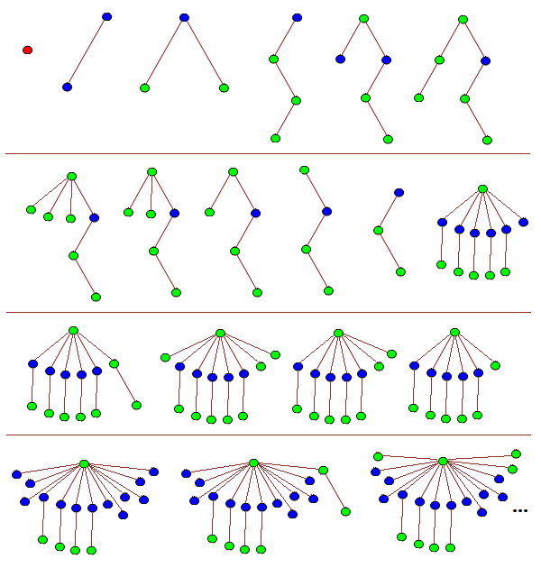
As you can see, by T_20 it’s getting difficult to draw the trees. A much more efficient notation is to use balanced parentheses:

T1 {}
T2 [[]]
T3 [()()]
T4 [((()))]
T5 ([(())][])
T6 ([(())](()))
T7 ([(())]()()())
T8 ([(())]()())
T9 ([(())]())
T10 ([(())])
T11 [(())]
T12 ([()][()][()][()][()][])
T13 ([()][()][()][()][()](()))
T14 ([()][()][()][()][()]()()())
T15 ([()][()][()][()][()]()())
T16 ([()][()][()][()][()]())
T17 ([()][()][()][()][()])
T18 ([()][()][()][()][][][][][][][][][])
T19 ([()][()][()][()][][][][][][][][](()))
T20 ([()][()][()][()][][][][][][][][]()()())
T21 ([()][()][()][()][][][][][][][][]()())
T22 ([()][()][()][()][][][][][][][][]())
T23 ([()][()][()][()][][][][][][][][])
...

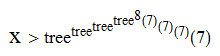
A related function, tree, asks for the longest sequence {U_1, U_2, …, U_tree(r)} of 1-labelled trees such that |U_n| ≤ n + r (for all n) and no tree is homeomorphically embeddable into a later tree. By extending the sequence shown above, it can be proved that TREE(3) has the following (weak) lower bound:

lowerbound

Proof (added 2020-07-24 in response to surprisingly hostile claims that I never had a proof of this bound): After the sequence described above, one can create a new tree, T24, which is of the form:

T24 ([()][()][()][()][][][][][][][]X7)

where X7 is any (monochromatically green) tree on 7 vertices. This can be followed by the sequence:

T25 ([()][()][()][()][][][][][][][]X8)
T26 ([()][()][()][()][][][][][][][]X9)
T27 ([()][()][()][()][][][][][][][]X10)
...

where X7, X8, X9, X10, … is a maximal-length sequence for tree(7). At the end of this process, we have:

T_(23 + tree(7)) ([()][()][()][()][][][][][][][]())

as () is necessarily the last element of the maximal-length sequence for tree(7). We can then extend the sequence further by ‘burning’ another blue node:

T_(24 + tree(7)) ([()][()][()][()][][][][][][][])
T_(25 + tree(7)) ([()][()][()][()][][][][][][]Y1)

where Y1 is the first tree in the maximal-length sequence for tree(tree(7)). We proceed in the same way as before with a sequence of tree(tree(7)) terms, culminating in:

T_(23 + tree(7) + tree(tree(7))) ([()][()][()][()][][][][][][]())
T_(24 + tree(7) + tree(tree(7))) ([()][()][()][()][][][][][][])
T_(25 + tree(7) + tree(tree(7))) ([()][()][()][()][][][][][]Y2)

where Y2 is the first tree in the maximal-length sequence for tree(tree(tree(7))). Repeating this process, we eventually reach the tree:

([()][()][()][()])

at time 24 + tree(7) + tree(tree(7)) + … + tree^8(7). We can then make the next tree in our process have the form:

([()][()][()][][][][][]...[]X7)

where we have created tree^8(7) new blue nodes by ‘burning’ a branch of the form [()]. The same argument as before allows us to reach the tree:

([()][()][()])

at time well beyond tree^(tree^8(7))(7). Repeating this outer iteration another three times gets us to the claimed bound.

To see that no tree embeds homeomorphically into a later tree, we note that if T precedes T’, then we have at least one of the following:

  • T contains more copies of [()] than T’;
  • T contains more copies of [] than T’;
  • The monochromatic green subtree of T precedes the monochromatic green subtree of T’;

where the latter condition was ensured by using a sequence for tree(k) which has this property by definition.

The result follows. QED

The game of Chomp

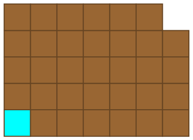
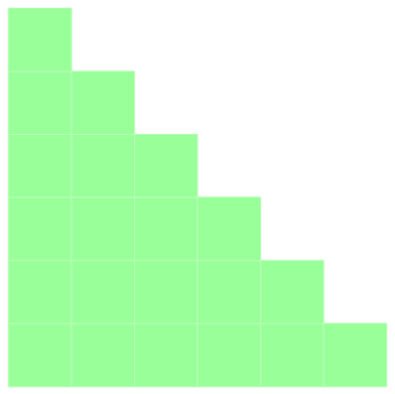
For a quick and refreshing detour from large numbers, we’ll consider the game of Chomp. We begin with a rectangular chocolate bar of size m by n, the bottom-left corner of which has been laced with cyanide.

chocolate

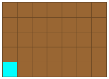
Players alternate turns, eating a square of chocolate together with everything above and to the right of it. For instance, after the first move the resulting configuration might resemble this:

chocolate3

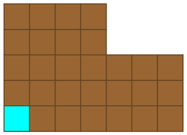
Then, the second player responds:

chocolate4

This continues until some unlucky person is left with the cyanide-laced square of chocolate and endures a slow, painful death. Who has the winning strategy? Without explicitly constructing a winning streategy, it’s possible to prove that the first player can force a win through an argument known as strategy stealing.

Assume that the second player has a winning strategy, with the intention of deriving a contradiction. Let the first player (I generally use Gabriel and Vishal as example names in combinatorial game theory, and we’ll use alphabetical order, so Gabriel) eat the top-right square of chocolate:

chocolate2

Now, Vishal has a winning strategy at this point. Let’s assume (without any real loss of generality) that he can force a win by making this move:

chocolate3

Gabriel could have made this move to begin with, so Vishal can’t possibly have a winning strategy. Reductio ad absurdum. As the game cannot terminate in a draw, we conclude that Gabriel has the winning strategy. This proof is heavily non-constructive, and no-one knows what this winning strategy is for arbitrary positive integers m,n.

Chomp is called an impartial game, since the same moves are theoretically available to each player, and it just depends on whose turn it is. Nim is another example. Both of these can be expressed as poset games, where players take turns to remove any element of a partially-ordered set together with all greater elements.

Making a game out of TREE(3)

That was a well-deserved distraction, but let’s return to TREE(3). We can define a two-player impartial game (which is, incidentally, a poset game) with the following rules:

  • Players alternate taking turns.
  • On the nth turn (odd for Gabriel, even for Vishal), each player draws a 3-labelled tree with at most n vertices.
  • If you draw a tree such that an earlier tree is homeomorphically embeddable into it, you lose.

By definition, such a game lasts at most TREE(3) turns and can never result in a draw. I don’t know what the parity of TREE(3) is, so I don’t know who wins the longest game. Indeed, I don’t even know which player has the winning strategy in TREE(3), and an exhaustive search is impractical. [Edited 2020-08-21: unfortunately, there’s a trivial winning strategy for the first player; after playing a single red vertex, respond to every move by your opponent by simply playing your opponent’s last tree with the colours blue and green reversed. An analogous game on subcubic graphs would be more interesting.]

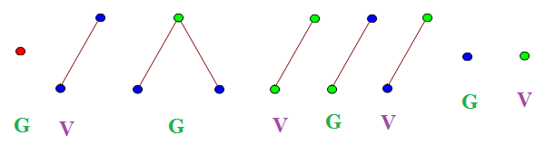
An example game is this one, which Vishal wins after 8 turns:

treegame

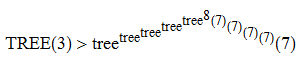
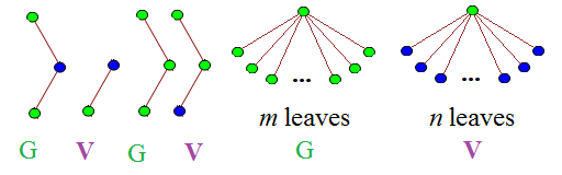
Believe it or not, all reasonably-sized games of Chomp can occur as positions in natural games of TREE(3). Firstly, we return to the previous scheme for getting really long sequences:

first20

Now, we can continue this for a very long time (x moves, where x has this unimaginably large lower bound):

Inequality for x

After this incredibly long sequence of moves, the next six moves might be these (let m and n be positive integers where m + n < x; in practice, x is so large that it is unrestrictive):

next6

This might not seem like a particularly poor move on Vishal’s part, but it transpires that Gabriel now has a definite winning strategy. If a player plays a single vertex (blue or green, since red was exhausted on the first move), the opponent can win by playing the single vertex of the other colour. Also note that no blue node can have a child, and no tree can have a depth more than three. In other words, subsequent moves resemble this:

four-three

This particular move is abbreviated to (4,3). Due to the ‘forbidden’ trees which appeared first, all moves must be of the form (a,b), where a < m and b < n. Interpreting these as coordinates, you may notice that this is precisely emulating the game of Chomp on a m by n grid! Exciting!

Consequently, Gabriel can force Vishal to ultimately play (0,0), which is a single green vertex. Gabriel immediately wins by playing a single blue vertex, leaving Vishal with no legal moves.

Posted in Activities, Fast-growing functions | 33 Comments

Cipher 8: Honeycomb

The inspiration for this cipher stemmed from a conversation with James Aaronson, when we considered the prospect of a whole new category of cipher. I was initially sceptical as to whether it could actually be implemented (they’re certainly much harder to design than to solve), but eventually settled upon the implementation below:

Click to enlarge

Click to enlarge

You’ll need the password (entirely lower-case, as has been the case since cipher #5) to access the solvers’ area. Good luck, and enjoy.

Posted in Ciphers | Leave a comment

Pictures of matchstick graphs

A matchstick graph is a planar graph with a plane embedding where all edges are of unit length. The name derives from the fact that they can be assembled on a flat surface out of matchsticks of equal length. Of particular interest are n-regular matchstick graphs. It’s easy to find 1-regular and 2-regular matchstick graphs (line segment and equilateral triangle, respectively). I’ll leave the case n = 3 as an exercise to the reader (it’s possible with 8 vertices and 12 edges, and not the first such graph you think of).

The smallest known 4-regular matchstick graph is the Harborth graph, with 52 vertices. It’s quite fun to make your own 4-regular matchstick graphs; mine ended up with 63 vertices:

4-regular graph

This has the additional property that the edges can be partitioned into 42 triangles, where each vertex is incident with two triangles. From this, it is therefore possible to derive a 3-regular planar graph of 42 vertices; this is obtained by doing the Δ-Y transform and contracting the resulting edges. Interestingly, this graph is itself a matchstick graph!

It has been proved that there are no finite 5-regular matchstick graphs, and the only 6-regular matchstick graph is the infinite triangular tiling (proof: consider Euler’s formula). On the surface of a sphere, however, the situation is different; there are a few 5-regular examples.

Snub polyhedra

The next object in this sequence is an infinite planar 5-regular matchstick graph.

Posted in Uncategorized | Leave a comment